Logistic Regression Optimization
In this module, I create my own toy dataset of 6 ultimate frisbee players, each rated on experience, skill, and athleticism. Each is also labeled as either a "good" or a "bad" player. I would like to teach a simple logistic regression model to predict whether a player is good or bad based on their experience, skill, and athleticism without using any machine learning libraries. Here we go!
1. Dataset
The toy dataset is defined in the file A1_Data_ILG.csv and is shown below:
import pandas as pd

df = pd.read_csv('A1_Data_ILG.csv')
print(df)
   experience  skill  athleticism label
0           5      8            5  good
1           4      4            3  good
2           2      2            4   bad
3           0      2            3   bad
4           5      6            5  good
5           1      0            0   bad
2. General Linear Equation
Let's define the general linear equation for a logistic regression model.
2a. $z = w_1 * x_1 + w_2 * x_2 + w_3 * x_3 + b$
2b. $z = w^T * x + b$
2c. The w values represent the weights of each of the inputs.
2d. The b value represents the bias.
3. Plot the Data
Let's take a look at this three dimensional data on a 3-dimensional plot.
# plot the data in A1_Data_ILG.csv

import pandas as pd
import matplotlib.pyplot as plt

# read the data
df = pd.read_csv('A1_Data_ILG.csv')

fig = plt.figure()
ax = plt.axes(projection='3d')

x1 = df['experience']
x2 = df['skill']
x3 = df['athleticism']
y = df['label']

# convert good to green and bad to red for the labels
y = y.replace('good', 'green')
y = y.replace('bad', 'red')

# plot the data with different colors for each label
ax.scatter3D(x1, x2, x3, s=100, c=y)

# add labels
ax.set_xlabel('experience')
ax.set_ylabel('skill')
ax.set_zlabel('athleticism')
ax.set_title('Simple 3D Dataset')

# show the plot
plt.show()

4. Visual Grouping
Let's look at the visual aspects of the data. The data does not appear to have strong clusters or groups, likely because there are only 7 data points and they are relatively dispersed. However, the data does seem linearly separable--all of the bad players are on the left, with the good players on the right.
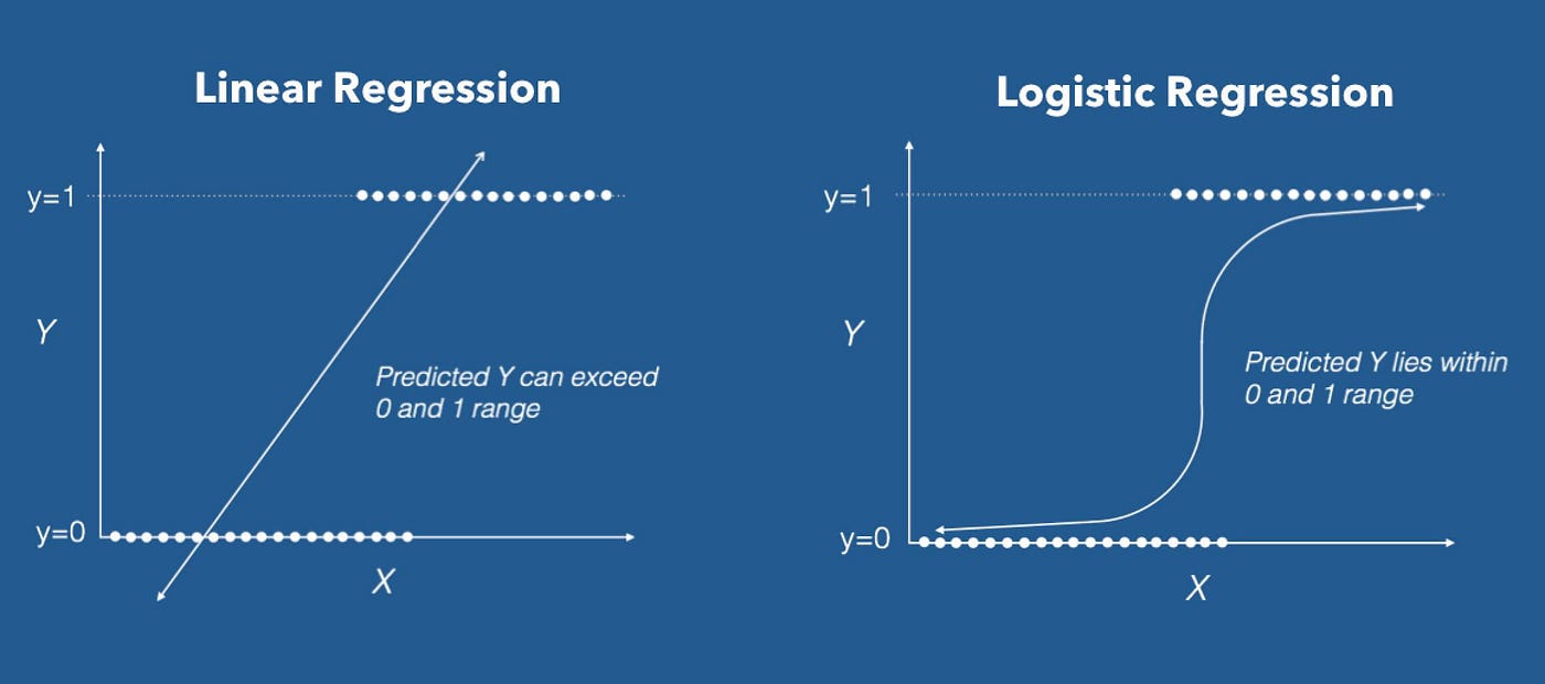
5. Sigmoid Function
In order to convert our linear predictions into a binary classification, let's transform the linear predictions using the sigmoid function as an activation function.
5a. The sigmoid function is defined as $1/(1+e^{-z})$ as well as $e^z/(1+e^z)$
5b. Let's prove that these are equivalent:
$$
\begin{align}
1/(1+e^{-z}) &= (1+e^z)/(1+e^z) * 1/(1+e^{-z}) \\
&= (1+e^z)/(1+e^z+e^z) \\
&= (1+e^z)/(1+e^z) * e^z/(1+e^z) \\
&= e^z/(1+e^z) \\
\end{align}
$$
Before we go any farther, let's normalize the data to have the maximum value in each column be 1 and the minimum value in each column be 0. This will make it easier to train the model.
# Normalize the Data

df = pd.read_csv('A1_Data_ILG.csv')

x1 = df['experience']
x2 = df['skill']
x3 = df['athleticism']
y = df['label']

df_norm = df.copy()
df_norm['experience'] = (x1 - x1.min()) / (x1.max() - x1.min())
df_norm['skill'] = (x2 - x2.min()) / (x2.max() - x2.min())
df_norm['athleticism'] = (x3 - x3.min()) / (x3.max() - x3.min())

df_norm.to_csv('A1_Data_ILG_norm.csv', index=False)

print('Normalized Data: \n', df_norm)
Normalized Data:
    experience  skill  athleticism label
0         1.0   1.00          1.0  good
1         0.8   0.50          0.6  good
2         0.4   0.25          0.8   bad
3         0.0   0.25          0.6   bad
4         1.0   0.75          1.0  good
5         0.2   0.00          0.0   bad
6. Run the First Epoch
Now let's get right into it! We're going to initialize the weight vector with 1s and the bias with 0, and run the first epoch.
6a. Weight vector: $[w_1, w_2, w_3] = [1, 1, 1]$
6b. Now we calculate the vector z:
math
 z  = w^T * x + b
    = [ 1.0,1.00,1.0,
        0.8,0.50,0.6,      [ 1,
        0.4,0.25,0.8,   *    1,  +  0
        0.0,0.25,0.6,        1 ]
        1.0,0.75,1.0,
        0.2,0.00,0.0 ]

    = [ 3.00,
        1.90,
        1.45,
        0.85,
        2.75,
        0.20 ]
6c. Now let's apply the activation function to get y^.
math
y^ = sigmoid(z)
    = 1/(1+e^-z) =
    = [ (1 + e^-3.00)^-1,
        (1 + e^-1.90)^-1,
        (1 + e^-1.45)^-1,
        (1 + e^-0.85)^-1,
        (1 + e^-2.75)^-1,
        (1 + e^-0.20)^-1 ]

    = [ 0.9526,
        0.8706,
        0.8101,
        0.7000,
        0.9404,
        0.5498 ]
6d. Finally, let's compare y^ with y.
math

  [ 1,
    1,
y = 0,
    0,
    1,
    0 ]

            [ 1,
              1,
y^(rounded) = 1,
              1,
              1,
              1 ]
Only 3 of the 6 predictions were correct, for rows 1, 2, and 5. This is a 50% accuracy rate, which is just as bad as randomly guessing. Therefore, y^ is not a good predictor of y.
6e. What's next? We can adjust our parameters w and b to improve our predictions. In order to determine how to adjust them, we can define a loss function to measure how far off y^ is from y. We can then find the gradient of the loss function with respect to our parameters, and change our parameters in the direction of the gradient to minimize the loss.
7. Loss Function
To improve our predictions, we're going to need to define how bad we did at predicting y. We can do this by defining a loss function. For this binary classification problem, we can use the Binary Cross Entropy Loss function.
7a. Binary Cross Entropy Function:
math
LCE(y^, y) = 1/N SUM_i^N {-yi * log(y^i) - (1-yi) * log(1-y^i)}
7b. Calculate the Binary Cross Entropy Loss for the first epoch:
math
LCE_1(y^1, y1) = - y1 * log(y^1) - (1-y1) * log(1-y^1) = - 1 * log(0.9526) - (1-1) * log(1-0.9526) = -log(0.9526) = 0.0482
LCE_2(y^2, y2) = - y2 * log(y^2) - (1-y2) * log(1-y^2) = - 1 * log(0.8706) - (1-1) * log(1-0.8706) = -log(0.8706) = 0.1386
LCE_3(y^3, y3) = - y3 * log(y^3) - (1-y3) * log(1-y^3) = - 0 * log(0.8101) - (1-0) * log(1-0.8101) = -log(0.1899) = 1.6613
LCE_4(y^4, y4) = - y4 * log(y^4) - (1-y4) * log(1-y^4) = - 0 * log(0.7000) - (1-0) * log(1-0.7000) = -log(0.3000) = 1.2040
LCE_5(y^5, y5) = - y5 * log(y^5) - (1-y5) * log(1-y^5) = - 1 * log(0.9404) - (1-1) * log(1-0.9404) = -log(0.9404) = 0.0614
LCE_6(y^6, y6) = - y6 * log(y^6) - (1-y6) * log(1-y^6) = - 0 * log(0.5498) - (1-0) * log(1-0.5498) = -log(0.4502) = 0.7981

LCE(y^, y) = 1/N SUM_i^N LCE_i = (0.0482 + 0.1386 + 1.6613 + 1.2040 + 0.0614 + 0.7981)/6 = 0.6519
7c. Given this, my current loss is my average cross entropy loss, 0.6519. This is not very good, as we want the LCE to approach 0. To improve this, I would adjust my weights and bias to get my predictions closer to the actual values. If the LCE is 0, that means that my predictions exactly match the actual values.
8. Try Again with New Weights
Before we methodically change our weights, let's take a guess at how to change them to reduce the loss. To do, I'll use domain knowledge. I know that skill, experience, and athleticism are all positively correlated with player rating, so I know that I want to keep my weights positive. All players only spanned a narrow range of predicted values, so I think I can increase my weights to differentiate them more. Every player was rated good in the last iteration, so I also need to adjust my bias downwards. I will then double the weights and try a bias of -3. I will try the following weights and bias:
math
w = [2, 2, 2]
b = -4
Recalculating the vector z:
math
 z  = w^T * x + b
    = [ 1.0,1.00,1.0,
        0.8,0.50,0.6,      [ 2,
        0.4,0.25,0.8,   *    2,  -  3
        0.0,0.25,0.6,        2 ]
        1.0,0.75,1.0,
        0.2,0.00,0.0 ]

    = [  3.0,
         0.8,
        -0.1,
        -1.3,
         2.5,
        -2.6 ]
Now apply the activation function to get y^.
math
y^ = sigmoid(z)
    = 1/(1+e^-z) =
    = [ (1 + e^-3.0)^-1,
        (1 + e^-0.8)^-1,
        (1 + e^0.1)^-1,
        (1 + e^1.3)^-1,
        (1 + e^-2.5)^-1,
        (1 + e^2.6)^-1 ]

    = [ 0.9526,
        0.6900,
        0.4750,
        0.2142,
        0.9241,
        0.0691 ]
Now recalculate the average loss using binary cross entropy:
math
LCE_2(y^2, y2) = - y2 * log(y^2) - (1-y2) * log(1-y^2) = - 1 * log(0.9526) - (1-1) * log(1-0.9526) = -log(0.9526) = 0.0486
LCE_1(y^1, y1) = - y1 * log(y^1) - (1-y1) * log(1-y^1) = - 1 * log(0.6900) - (1-1) * log(1-0.6900) = -log(0.6900) = 0.3711
LCE_3(y^3, y3) = - y3 * log(y^3) - (1-y3) * log(1-y^3) = - 0 * log(0.4750) - (1-0) * log(1-0.4750) = -log(0.5250) = 0.6444
LCE_4(y^4, y4) = - y4 * log(y^4) - (1-y4) * log(1-y^4) = - 0 * log(0.2142) - (1-0) * log(1-0.2142) = -log(0.7858) = 0.2410
LCE_5(y^5, y5) = - y5 * log(y^5) - (1-y5) * log(1-y^5) = - 1 * log(0.9241) - (1-1) * log(1-0.9241) = -log(0.9241) = 0.0789
LCE_6(y^6, y6) = - y6 * log(y^6) - (1-y6) * log(1-y^6) = - 0 * log(0.0691) - (1-0) * log(1-0.0691) = -log(0.9309) = 0.0716

LCE(y^, y) = 1/N SUM_i^N LCE_i = (0.0486 + 0.3711 + 0.6444 + 0.2410 + 0.0789 + 0.0716)/6 = 0.2426
My new loss is 0.2426, which is much better than my previous loss of 0.6519. This means that my predictions are much closer to the actual values, so I was right about how to change my weights!
9. Calculate the Gradient
Okay, now it's time to improve our predictions methodically. To do this, we need to calculate the gradient of the loss function with respect to our parameters. We can then change our parameters in the direction of the gradient to minimize the loss.
9a1. Find the partial derivate of the LCE with respect to the weight vector w:
math
dLCE/dw = dLCE/dy^ * dy^/dz * dz/dw

    dLCE/dy^= d/dy^ (1/N (-y * log(y^) - (1-y) * log(1-y^)))
            = 1/N (-y * (1/y^) - (1-y) * (-1/(1-y^)))
            = 1/N (-y/y^ + (1-y)/(1-y^))

    dy^/dz = d/dz (1/(1+e^-z))
           = d/dz (1+e^-z)^-1
           = -(1+e^-z)^-2 * d/dz (1+e^-z)
           = -(1+e^-z)^-2 * -e^-z
           = e^-z/(1+e^-z)^2
           = 1/(1+e^-z) * e^-z/(1+e^-z)
           = y^ * (1+e^-z-1)/(1+e^-z)
           = y^ * (1-y^)

     dz/dw = d/dw (w^T * x + b)
           = x

dLCE/dw = dLCE/dy^ * dy^/dz * dz/dw
        = 1/N (-y/y^ + (1-y)/(1-y^)) * y^ * (1-y^) * x
        = 1/N (-y*y^*(1-y)/y^ + (1-y)*y^*(1-y^)/(1-y^)) * x
        = 1/N (-y*(1-y) + (1-y)*y^) * x
        = 1/N (-y + y^y + y^ - y^y) * x
        = 1/N (y^ - y)^T * x

dLCE/dw = 1/N (y^ - y)^T * x
9a2. Find the partial derivate of the LCE with respect to the bias b:
math

dLCE/db = dLCE/dy^ * dy^/dz * dz/db

  dLCE/dy^ = 1/N (-y/y^ + (1-y)/(1-y^))

    dy^/dz = y^ * (1-y^)

     dz/db = d/db (w^T * x + b)
           = 1

dLCE/db = dLCE/dy^ * dy^/dz * dz/dw
        = 1/N (-y/y^ + (1-y)/(1-y^)) * y^ * (1-y^) * 1
        = 1/N (y^ - y) * 1

dLCE/db = 1/N (y^ - y)
9b. What do these derivatives mean in a few sentences?
9b1. The partial derivative of the loss function with respect to w is proportional to:
- The difference between the predicted value and the actual value -- the closer these two values are, the smaller the derivative will be. This makes sense since that's our objective. It also flips the sign of the gradient if we overshoot in our prediction.
- The input value X -- the smaller the input value, the smaller the derivative will be. This makes sense since the smaller the input value, the less it will affect the output value, so the less we want to change the weight. Also, if it's negative, it will flip the direction of the gradient.
9b2. The partial derivative of the loss function with respect to b is proportional to:
- The first above factor
- It does not depend on the input value X, since the bias term isn't multiplied by the inputs.
10. Run the Second Epoch with Gradient Descent
Now that we have our gradients, we can use them to update our weights. For now for simplicity, we won't update the bias.
10a. Calculate the new weights given the gradient and learning rate of 1:
math
dLCE/dw = 1/N (y^ - y)^T * x

        y^ - y = [ 0.9526, 0.8699, 0.8100, 0.7006, 0.9399, 0.5498 ] - [ 1, 1, 0, 0, 1, 0 ] = [ -0.0474, -0.1301, 0.8100, 0.7006, -0.0601, 0.5498 ]

dLCE/dw = 1/6 * [ -0.0474, -0.1301, 0.8100, 0.7006, -0.0601, 0.5498 ] * [1	1	1
                                                                         0.8	0.5	0.6
                                                                         0.4	0.25	0.8
                                                                         0	0.25	0.6
                                                                         1	0.75	1
                                                                         0.2	0	0   ]

        = 1/6 * [0.2224, 0.2201, 0.8828]
        = [0.0371, 0.0367, 0.1471]

w2 = w1 - LR * dLCE/dw
   = [1, 1, 1] - 1 * [0.0371, 0.0367, 0.1471]
   = [0.9629, 0.9633, 0.8529]
10b. Run another epoch with the updated weights.
Given the new weights w2, calculate the new z values:
math
 z  = w^T * x + b
    = [ 1.0,1.00,1.0,
        0.8,0.50,0.6,      [ 0.9629,
        0.4,0.25,0.8,   *    0.9633,  -  0
        0.0,0.25,0.6,        0.8529 ]
        1.0,0.75,1.0,
        0.2,0.00,0.0 ]

    = [ 2.7791,
        1.7637,
        1.3083,
        0.7526,
        2.5383,
        0.1926 ]
Given the new z values, calculate the new y^ values:
math
y^ = sigmoid(z)
    = 1/(1+e^-z) =
    = [ (1 + e^-2.7791)^-1,
        (1 + e^-1.7637)^-1,
        (1 + e^-1.3083)^-1,
        (1 + e^-0.7526)^-1,
        (1 + e^-2.5383)^-1,
        (1 + e^-0.1926)^-1 ]

    = [ 0.9415,
        0.8537,
        0.7872,
        0.6797,
        0.9268,
        0.5480 ]
Given the new y^ values, calculate the new LCE:
math
LCE_1(y^1, y1) = - y1 * log(y^1) - (1-y1) * log(1-y^1) = - 1 * log(0.9415) - (1-1) * log(1-0.9415) = -log(0.9415) = 0.0602
LCE_2(y^2, y2) = - y2 * log(y^2) - (1-y2) * log(1-y^2) = - 1 * log(0.8537) - (1-1) * log(1-0.8537) = -log(0.8537) = 0.1582
LCE_3(y^3, y3) = - y3 * log(y^3) - (1-y3) * log(1-y^3) = - 0 * log(0.7872) - (1-0) * log(1-0.7872) = -log(0.2128) = 1.5475
LCE_4(y^4, y4) = - y4 * log(y^4) - (1-y4) * log(1-y^4) = - 0 * log(0.6797) - (1-0) * log(1-0.6797) = -log(0.3203) = 1.1386
LCE_5(y^5, y5) = - y5 * log(y^5) - (1-y5) * log(1-y^5) = - 1 * log(0.9268) - (1-1) * log(1-0.9268) = -log(0.9268) = 0.0760
LCE_6(y^6, y6) = - y6 * log(y^6) - (1-y6) * log(1-y^6) = - 0 * log(0.5480) - (1-0) * log(1-0.5480) = -log(0.4520) = 0.7941

LCE(y^, y) = 1/N SUM_i^N LCE_i = (0.0602 + 0.1582 + 1.5475 + 1.1386 + 0.0760 + 0.7941)/6 = 0.6291
10c. My new loss after updating the weights is 0.6291, which is better than the original loss of 0.6519! This is really interesting since I think that larger weights would actually improve the loss, as shown in problem #8. However, it seems that smaller weights improved the loss because it brought the predictions closer to 0, which brought bad players closer to negative z values. I suspect that the weights will get smaller and smaller until the bias term is negative enough, then the weights will increase. I hope that's actually the case when I code it with more epochs below!
11. Hand Code a Logistic Regression Model
Now for the fun part! Instead of doing math by hand, we're going to let Python do the math for us. We're going to code a logistic regression model from scratch! The requirements of this code are as follows:
(a) Read in any .csv labeled dataset where the Label is called "LABEL".
(b) The code should create "y" (the label) as a numpy array of 0 and 1. So, if the labels are originally something like POS and NEG, you r code will need to determine this, and then update all POS to 1 and all NEG to 0. The code should be able to do this for any two label options.
(c) The code will also create X which is the entire dataset (without the labels) as a numpy array.
(d) The code will initialize w and b and a learning rate.
(e) The code will need to contain a function for Sigmoid and for z, etc.
(f) The code will then need to perform gradient descent to optimize (reduce) LCE.
(g) Be sure that the code can run iteratively for as many epochs as you wish.
(h) Show a final confusion matrix AND show a graph of how the LCE reduces as epochs iterate.
Recommended: Use the code to see if your by-hand results from above are right.
import numpy as np
import pandas as pd
import matplotlib.pyplot as plt

def read_data(path):
    """read in data from a file path
    path is a string pointing to a local directory
    the data file should be a csv
    if debug >= 1:
        prints the top rows of the datafile
    returns a pandas dataframe of the csv
    """
    if debug >= 1:
        print('Reading in data from ' + path + '...')
    df = pd.read_csv(path)
    if debug >= 2:
        print('Data loaded. Here is a sneak peak: \n', df.head())
    return df


def clean_data(df):
    """clean the data
    Takes in a dataframe df
    Returns two numpy arrays x and y
    x is inputs normalized between 0-1
    y is labels converted to 0 or 1
    """
    if debug >= 1:
        print('Now cleaning the data.')
    # get the size of the matrix
    nrows = df.shape[0]
    ncols = df.shape[1]
    if debug >= 2:
        print('The shape of the data is: ', df.shape)

    # intialize x and y
    x = np.empty((nrows,ncols-1))
    y = np.empty((nrows,1))

    # separate labels
    if 'LABEL' in df.columns:
        y = np.array(df['LABEL'])
        x = np.array(df[df.columns.difference(['LABEL'])])
    elif 'label' in df.columns:
        y = np.array(df['label'])
        x = np.array(df[df.columns.difference(['label'])])
    else:
        raise Exception('There is no column with the title label in the data')
    if debug >= 2:
        print('x is: \n', x)
    if debug >= 2:
        print('y is: \n', y)

    # convert labels to 0 or 1
    y = convert_labels(y)
    # convert shape from 1D array to 2D with 1 column
    y = y.reshape(-1, 1)
    if debug >= 2:
        print('New y is : \n', y)

    # normalize x
    x = normalize(x)
    if debug >= 2:
        print('New x is : \n', x)

    # return x and y
    return x, y


def convert_labels(y):
    """converts y labels
    accepts in a numpy array with binary values
    converts the first value to 0, all others to 1
    returns a numpy array of 0s and 1s
    """
    if debug >= 1:
        print('Converting labels to 0,1...')
    y_values = set(y)
    y_value_0 = list(y_values)[0]
    y_value_1 = list(y_values)[1]

    y[y == y_value_0] = 0
    y[y == y_value_1] = 1
    return y

def normalize(x):
    """normalizes x values
    accepts a numpy array of floats
    converts them to a max of 1 and min of 0
    returns a numpy array
    """
    if debug >= 1:
        print('Normalizing x values...')
    xrows = x.shape[0]
    xcols = x.shape[1]
    xnorm = np.empty((xrows, xcols))
    for j, column in enumerate(x.T):
        max = column.max()
        min = column.min()
        for i, item in enumerate(column):
            xnorm[i,j] = (item - min)/(max - min)
    return xnorm

def logistic_regression(x, y, learning_rate = 0.1, epochs = 100):
    """run logistic regression on the input data
    accepts the inputs, labels, LR, and # of epochs
    runs logistic regression for the given number of epochs
    graphs the error rate over time
    graphs the confusion matrix for the final predictions
    """
    if debug >= 1:
        print('Running logistic regression...')

    # inspect shape of data
    xrows = x.shape[0]
    xcols = x.shape[1]
    yrows = y.shape[0]
    ycols = y.shape[1]

    # validate y is N x 1 dimensions
    if yrows != xrows:
        raise Exception('The size of the label vector does not match the input data')
    if ycols != 1:
        raise Exception('The label vector should only have 1 column')

    # create arrays to store losses
    cols = []
    for i in range(xcols):
        cols.append('w' + str(i+1))
    cols.append('b')
    cols.append('lce_avg')
    weights_df = pd.DataFrame(columns = cols)

    # initialize the weights and the bias
    w = np.ones((1, xcols))
    b = 0
    if debug >= 2:
        print('The initial weights are: \n', w)
    if debug >= 2:
        print('The initial bias is: ', b)

    for e in range(epochs+1):

        # log current weights
        new_weight_row = []
        for i, weight in enumerate(w[0]):
            new_weight_row.append(weight)
        new_weight_row.append(b)
        new_weight_row.append(0) # placeholder for loss later
        weights_df.loc[len(weights_df)] = new_weight_row
        if debug >= 2:
            print('The weights_df is now:\n', weights_df)

        # compute z = x * w^T + b
        z = x @ w.T + b
        z = z.astype(float)
        if debug >= 2:
            print('The z vector is: \n', z)

        y_hat = 1 / ( 1 + np.exp(-z) )
        if debug >= 2:
            print('The y_hat is: \n', y_hat)

        # calculate the loss with binary cross entropy
        lce = (- y * np.log(y_hat) - (1-y) * np.log(1-y_hat))
        lce_avg = 1/xrows * np.sum(lce)
        weights_df['lce_avg'][e] = lce_avg
        if debug >= 2:
            print('The loss is \n:', lce_avg)

        # calculate the gradient for w
        dlce_dw = 1/xrows * (y_hat - y).T @ x
        if debug >= 2:
            print('The weight gradient is: ', dlce_dw)

        # update the weights
        dw = dlce_dw * learning_rate
        w = w - dw
        if debug >= 2:
            print('The new weights are: ', w)

        # calculate the gradient for b
        dlce_db = 1/xrows * np.sum(y_hat - y)
        if debug >= 2:
            print('The bias gradient is: ', dlce_db)

        # update the bias
        db = dlce_db * learning_rate
        b = b - db
        if debug >= 2:
            print('The new bias is :', b)

        # repeat for e epochs
    if export == 1:
        weights_df.to_csv('A1_Weights_ILG.csv', index=False)
    return weights_df, y_hat

def plot_results(weights_df, y_hat, y):
    '''plot the results of the logistic regression
    takes in a dataframe with n weights, the bias, and loss for each epoch
    plots the error over time
    plots the weights and bias over time
    plots the confusion matrix for the final result
    '''
    # plot the error over each epoch from the index column
    if debug >= 1:
        print('Plotting the error over time...')
    _, ax = plt.subplots()
    ax.plot(weights_df.index, weights_df['lce_avg'])
    ax.set_xlabel('Epochs')
    ax.set_ylabel('Loss')
    ax.set_title('Loss over time')
    plt.show()

    # plot the weights and bias over time
    if debug >= 1:
        print('Plotting the weights over time...')
    _, ax = plt.subplots()
    for column in weights_df.columns[:-1]:
        ax.plot(weights_df.index, weights_df[column])
    ax.set_xlabel('Epochs')
    ax.set_ylabel('Weights')
    ax.set_title('Weights over time')
    # add legend
    ax.legend(weights_df.columns[:-1])
    plt.show()

    # plot a confusion matrix of y_hat vs y
    if debug >= 1:
        print('Plotting the confusion matrix...')
    y_hat = y_hat.round()
    y_hat = y_hat.astype(int)
    y = y.astype(int)
    confusion_matrix = pd.crosstab(y_hat[:,0], y[:,0], rownames=['Predicted'], colnames=['Actual'])
    # create a plot of the confusion matrix with a 2x2 grid with colors
    _, ax = plt.subplots()
    ax.matshow(confusion_matrix, cmap=plt.cm.Blues)
    # add labels
    ax.set_xlabel('Actual')
    ax.set_ylabel('Predicted')
    # add numbers
    for i in range(2):
        for j in range(2):
            ax.text(j, i, confusion_matrix.iloc[i, j], ha='center', va='center', color='green')
    plt.show()

    # print the weights
    if debug >= 2:
        print('Full weight evolution: \n', weights_df)
    return

def main():
    """main function
    Entrypoint to the file
    Calls all other functions
    """
    df = read_data('A1_Data_ILG.csv')
    x, y = clean_data(df)
    LR = 25
    epochs = 20
    weights_df, y_hat = logistic_regression(x, y, LR, epochs)
    plot_results(weights_df, y_hat, y)
    return

# set debug level
# 0 = print nothing
# 1 = print important statements
# 2 = print all statements
debug = 1
export = 1

# call of the code above!
main()
Reading in data from A1_Data_ILG.csv...
Now cleaning the data.
Converting labels to 0,1...
Normalizing x values...
Running logistic regression...
Plotting the error over time...

Plotting the weights over time...

Plotting the confusion matrix...

Conclusion
That's it, we did it! If we look at the confusion matrix, we can see that we correctly predicted 6 out of 6 players, which is an 100% accuracy rate! Not a huge suprise since the data were clearly linearly separable as we saw in the visualization earlier. Still, not bad for a hand-coded optimization algorithm!
This example illustrates how a single node in a neural network operates by taking in inputs, applying a linear transformation to each one, activating the result of that transformation into an output prediction, calculating the error from the predicted values to the truth, and then adjusting the weights and bias to minimize the error. This is the basis of all neural networks! Thanks for reading.
P.S. The code below is for exporting this Jupyter notebook into HTML for this website.
# export to HTML for webpage
import os

# os.system('jupyter nbconvert --to html mod1.ipynb')
os.system('jupyter nbconvert --to html mod1.ipynb --HTMLExporter.theme=dark')
[NbConvertApp] Converting notebook mod1.ipynb to html
[NbConvertApp] Writing 795339 bytes to mod1.html
0