Simple Neural Networks
Part 1: Single Hidden Layer with Sigmoid Activation Function
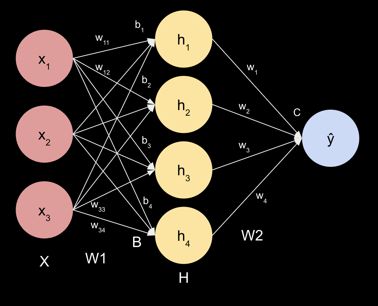
#1: Illustration of the Matrices Associated with the Neural Network
$X = \begin{bmatrix} x_1 & x_2 & x_3 \end{bmatrix}$
$W1 = \begin{bmatrix} w_{11} & w_{21} & w_{31}\\ w_{12} & w_{22} & w_{32}\\ w_{13} & w_{23} & w_{33}\\ w_{14} & w_{24} & w_{34}\\ \end{bmatrix}$
$H = \begin{bmatrix} h_1\\ h_2\\ h_3\\ h_4\\ \end{bmatrix}$
$W2 = \begin{bmatrix} w_{11} & w_{21} & w_{31} & w_{41}\\ \end{bmatrix}$
$B = \begin{bmatrix} b_1 & b_2 & b_3 & b_4 \end{bmatrix}$
$C \in \mathbb{R}$ (c is a scalar)
$Z1 = X * W1.T + B = \begin{bmatrix} z_1\\ z_2\\ z_3\\ z_4\\ \end{bmatrix}$
$\sigma (z) = \frac{1}{1+e^{-z}}$
$H = \sigma(Z1)$
$Z2 = H * W2.T + C$ (scalar)
$\hat{y} = \sigma(Z2)$ (scalar)
$y \in \mathbb{R}$ (scalar)
$\hat{y} - y \in \mathbb{R} $ (scalar)
Assuming binary cross entropy:
$L = -y\log(\hat{y}) - (1-y)\log(1-\hat{y})$ (scalar)
With Mean Squared Error:
$L = \frac{1}{N}\sum{(\hat{y} - y)^2}$ (scalar)
#2: Python to Code the Feed Forward portion of this Neural Network
a-c. Create a dataset and read it in (raw dataset is here)
#2a-c: Create and read in dataa
import numpy as np

np.set_printoptions(precision=6)

def get_xy(df):

    nrows = df.shape[0]
    ncols = df.shape[1]

    x = np.empty((nrows,ncols-1))
    y = np.empty((nrows,1))

    # separate labels
    if 'LABEL' in df.columns:
        y = np.array(df['LABEL'])
        x = np.array(df[df.columns.difference(['LABEL'])])
    elif 'label' in df.columns:
        y = np.array(df['label'])
        x = np.array(df[df.columns.difference(['label'])])
    else:
        raise Exception('There is no column with the title label in the data')
    return x, y

def binary_labels(y):
    y_values = set(y)
    y_value_0 = list(y_values)[0]
    y_value_1 = list(y_values)[1]
    y[y == y_value_0] = 0
    y[y == y_value_1] = 1
    y = y.reshape(-1, 1)
    return y.astype(int)

def normalize(x):
    xrows = x.shape[0]
    xcols = x.shape[1]
    xnorm = np.empty((xrows, xcols))
    for j, column in enumerate(x.T):
        max = column.max()
        min = column.min()
        for i, item in enumerate(column):
            xnorm[i,j] = (item - min)/(max - min)
    return xnorm.astype(float)
import pandas as pd
df = pd.read_csv('A2_Pt1_Data_ILG.csv')
x, y = get_xy(df)
y = binary_labels(y)
x = normalize(x)

print('Data is: \n', df)
print('x is: \n', x)
print('y is: \n', y)
Data is:
    experience  skill  athleticism label
0           5      8            5  good
1           4      4            3  good
2           2      2            4   bad
3           0      2            3   bad
4           5      6            5  good
5           1      0            0   bad
x is:
 [[1.   1.   1.  ]
 [0.6  0.8  0.5 ]
 [0.8  0.4  0.25]
 [0.6  0.   0.25]
 [1.   1.   0.75]
 [0.   0.2  0.  ]]
y is:
 [[0]
 [0]
 [1]
 [1]
 [0]
 [1]]
import numpy as np
import pandas as pd

#2d: Code a sigmoid function and the derivative
def sigmoid(z):
    return 1/(1+np.exp(-z))

def sigmoid_derivative(z):
    return sigmoid(z) * (1-sigmoid(z))

#2e: Code the loss function
def mse(y, y_hat):
    return np.square(y - y_hat).mean()

def mse_derivative(y, y_hat):
    return -2*(y - y_hat)

#2: Code the feedforward function
class NeuralNetwork3D():

    def __init__(self, LR=0.1, epochs=10):
        self.LR = LR
        self.epochs = epochs
        # shape parameters
        # hidden_layers = 1
        self.hidden_layer_dim = 4
        self.output_layer_dim = 1
        self.input_layer_dim = 3

        # initialize with w1 = 1, b = 0, w2 = 2, c = -1
        self.w1 = np.ones((self.hidden_layer_dim, self.input_layer_dim))
        self.b = np.zeros((1, self.hidden_layer_dim))
        self.w2 = 2 * np.ones((self.output_layer_dim, self.hidden_layer_dim))
        self.c = -1 * np.ones((1, self.output_layer_dim))

    def randomize_weights(self):
        np.random.seed(44)
        self.w1 = np.random.rand(self.hidden_layer_dim, self.input_layer_dim)
        self.b = np.random.rand(1, self.hidden_layer_dim)
        self.w2 = np.random.rand(self.output_layer_dim, self.hidden_layer_dim)
        self.c = np.random.rand(1, self.output_layer_dim)

    def feed_forward(self, x):
        self.z1 = (x @ self.w1.T + self.b).astype(float)
        self.h = sigmoid(self.z1).astype(float)
        self.z2 = (self.h @ self.w2.T + self.c).astype(float)
        self.y_hat = sigmoid(self.z2).astype(float)
        return

    def calculate_loss(self, y):
        self.loss = mse(y, self.y_hat).astype(float)
        return

    def print_params(self):
        print('\nW1 is: \n', self.w1)
        print('\nB is: \n', self.b)
        print('\nZ1 is: \n', self.z1)
        print('\nH is: \n', self.h)
        print('\nW2 is: \n', self.w2)
        print('\nZ2 is: \n', self.z2)
        print('\nC is: \n', self.c)
        print('\ny^ is: \n', self.y_hat)
        print('\nL is: \n', self.loss)

# test code
# nn1 = NeuralNetwork3D()
# nn1.feed_forward(x)
# nn1.calculate_loss(y)
# nn1.print_params()
#3: Check the Feed Forward Math Above by Hand
Use just the first row of the dataset, assume W1 is 1, W2 is 2, b is 0, and c is -1. Check it against the code above.
#3.1: Run a Feed Forward Iteration by Hand
$X = \begin{bmatrix} x_1 & x_2 & x_3 \end{bmatrix} = \begin{bmatrix} 1 & 1 & 1 \end{bmatrix} $
$W1 = \begin{bmatrix} w_{11} & w_{21} & w_{31}\\ w_{12} & w_{22} & w_{32}\\ w_{13} & w_{23} & w_{33}\\ w_{14} & w_{24} & w_{34}\\ \end{bmatrix} = \begin{bmatrix} 1 & 1 & 1\\ 1 & 1 & 1\\ 1 & 1 & 1\\ 1 & 1 & 1\\ \end{bmatrix}$
$Z1 = X * W1.T + B = \begin{bmatrix} z_1\\ z_2\\ z_3\\ z_4\\ \end{bmatrix} = \begin{bmatrix} x_1*w_{11} + x_2*w_{21} + x_3*w_{31} + b_1\\ x_2*w_{12} + x_2*w_{22} + x_3*w_{32} + b_2\\ x_3*w_{13} + x_2*w_{23} + x_3*w_{33} + b_3\\ x_4*w_{14} + x_2*w_{24} + x_3*w_{34} + b_4\\ \end{bmatrix} = \begin{bmatrix} 1*1 + 1*1 + 1*1 + 0\\ 1*1 + 1*1 + 1*1 + 0\\ 1*1 + 1*1 + 1*1 + 0\\ 1*1 + 1*1 + 1*1 + 0\\ \end{bmatrix} = \begin{bmatrix} 3\\ 3\\ 3\\ 3\\ \end{bmatrix}$
$H = \begin{bmatrix} h_1\\ h_2\\ h_3\\ h_4\\ \end{bmatrix} = \begin{bmatrix} \sigma(z_1)\\ \sigma(z_2)\\ \sigma(z_3)\\ \sigma(z_4)\\ \end{bmatrix} = \begin{bmatrix} \frac{1}{1+e^{-z_1}}\\ \frac{1}{1+e^{-z_2}}\\ \frac{1}{1+e^{-z_3}}\\ \frac{1}{1+e^{-z_4}}\\ \end{bmatrix} = \begin{bmatrix} \frac{1}{1+e^{3}}\\ \frac{1}{1+e^{3}}\\ \frac{1}{1+e^{3}}\\ \frac{1}{1+e^{3}}\\ \end{bmatrix} = \begin{bmatrix} 0.952574\\ 0.952574\\ 0.952574\\ 0.952574\\ \end{bmatrix} $
$W2 = \begin{bmatrix} w_{11} & w_{21} & w_{31} & w_{41}\\ \end{bmatrix} = \begin{bmatrix} 2 & 2 & 2 & 2\\ \end{bmatrix}$
$B = \begin{bmatrix} b_1\\ b_2\\ b_3\\ b_4\\ \end{bmatrix} = \begin{bmatrix} 0\\ 0\\ 0\\ 0\\ \end{bmatrix}$
$C = -1$
$Z2 = W2 * H + C = \begin{bmatrix} 2 & 2 & 2 & 2\\ \end{bmatrix} * \begin{bmatrix} 0.952574\\ 0.952574\\ 0.952574\\ 0.952574\\ \end{bmatrix} - 1 = 6.620593 $
$\hat{y} = \sigma(Z2) = \sigma(6.620593) = \frac{1}{1+e^{-6.620593}} = 0.998669$
$y = 1$
$y - \hat{y} = 0.001331$
Mean Squared Error:
$L = \frac{1}{N}\sum{(\hat{y} - y)^2} = \frac{1}{1}(0.001331)^2 = 0.00000177$
#3.2: Run a Feed Forward Iteration by Code
# extract just the first row of data
x0 = x[0]
y0 = y[0]

# run through the neural network nn1
nn1 = NeuralNetwork3D()
nn1.feed_forward(x0)
nn1.calculate_loss(y0)

# Print out X, y, W1, B, Z1, H1, W2, Z2, C, y^, y^-y, and L.
print('X is: \n', x0)
print('\ny is: \n', y0)
nn1.print_params()
print('\ny-y^ is: \n', y0 - nn1.y_hat)
X is:
 [1. 1. 1.]

y is:
 [0]

W1 is:
 [[1. 1. 1.]
 [1. 1. 1.]
 [1. 1. 1.]
 [1. 1. 1.]]

B is:
 [[0. 0. 0. 0.]]

Z1 is:
 [[3. 3. 3. 3.]]

H is:
 [[0.952574 0.952574 0.952574 0.952574]]

W2 is:
 [[2. 2. 2. 2.]]

Z2 is:
 [[6.620593]]

C is:
 [[-1.]]

y^ is:
 [[0.998669]]

L is:
 0.9973400374685585

y-y^ is:
 [[-0.998669]]
The key results, namely $\hat{y}$ and $L$ are the same as the hand calculation above. Hooray!
#4: Write out the derivatives for each of the parameters in the Neural Network
Partial derivative of L with respect to C: $ \frac{\partial L}{\partial C} \\ \quad = \frac{\partial L}{\partial \hat{y}} * \frac{\partial \hat{y}}{\partial Z2} * \frac{\partial Z2}{\partial C} \\ \quad = \frac{1}{N}*-2(y-\hat{y}) * \hat{y}(1-\hat{y}) * 1 \\ \quad = -\frac{2}{N}*(y-\hat{y})*\hat{y}(1-\hat{y}) \\ $
Partial derivative of L with respect to W2: $ \frac{\partial L}{\partial W2} \\ \quad = \frac{\partial L}{\partial \hat{y}} * \frac{\partial \hat{y}}{\partial Z2} * \frac{\partial Z2}{\partial B} \\ \quad = \frac{1}{N}*-2(y-\hat{y}) * \hat{y}(1-\hat{y}) * H \\ \quad = -\frac{2}{N}*(y-\hat{y})*\hat{y}(1-\hat{y})*H \\ \quad = \frac{\partial L}{\partial C}*H $
Partial derivative of L with respect to B: $ \frac{\partial L}{\partial B} \\ \quad = \frac{\partial L}{\partial \hat{y}} * \frac{\partial \hat{y}}{\partial Z2} * \frac{\partial Z2}{\partial H} * \frac{\partial H}{\partial Z1} * \frac{\partial Z1}{\partial B} \\ \quad = \frac{1}{N}*-2(y-\hat{y}) * \hat{y}(1-\hat{y}) * W2 * H(1-H) * 1 \\ \quad = -\frac{2}{N}*(y-\hat{y})*\hat{y}(1-\hat{y})*W2*H(1-H) \\ \quad = \frac{\partial L}{\partial C}*W2*H(1-H) $
Partial derivative of L with respect to W1: $ \frac{\partial L}{\partial W1} \\ \quad = \frac{\partial L}{\partial \hat{y}} * \frac{\partial \hat{y}}{\partial Z2} * \frac{\partial Z2}{\partial H} * \frac{\partial H}{\partial Z1} * \frac{\partial Z1}{\partial W1} \\ \quad = \frac{1}{N}*-2(y-\hat{y}) * \hat{y}(1-\hat{y}) * W2 * H(1-H) * X \\ \quad = -\frac{2}{N}*(y-\hat{y})*\hat{y}(1-\hat{y})*W2*H(1-H)*X \\ \quad = \frac{\partial L}{\partial C}*W2*H(1-H)*X \\ \quad = \frac{\partial L}{\partial B}*X $
#5: Code Backpropogation
# assume x and y have been read
# assume mse and sigmoid have been defined
# assume np has been imported
# assume NeuralNetwork3D class has been defined

import matplotlib.pyplot as plt
from sklearn.metrics import confusion_matrix, ConfusionMatrixDisplay

def update_weights(self, y):
    self.dLdC = (2*(mse_derivative(y, self.y_hat) * sigmoid_derivative(self.z2))).astype(float) # shape is (6x1)
    self.dLdW2 = (self.dLdC * self.h).astype(float) # (6x1)*(6x4) = (6x4)
    self.dLdB = (self.dLdC @ self.w2).astype(float) * sigmoid_derivative(self.z1) # (6x1) @ (1x4) * (6x4) = (6x4)
    self.dLdW1 = (self.dLdB.T @ x).astype(float) # (4x6) @ (6x3) = (4x3)
    self.c = (self.c - self.LR * self.dLdC.mean()).astype(float) # (1x1) - LR*(6x1).mean = (1x1)
    self.w2 = (self.w2 - self.LR * self.dLdW2.mean(axis=0)).astype(float) # (1x4) - LR*(6x4).mean = (1x4)
    self.b = (self.b - self.LR * self.dLdB.mean(axis=0)).astype(float) # (1x4) - LR*(6x4).mean = (1x4)
    self.w1 = (self.w1 - self.LR * self.dLdW1).astype(float) # (4x3) - LR*(4x3) = (4x3)
    return

def print_derivatives(self):
    # print derivatives rounded to 5 decimal places
    print('\ndLdC is: \n', self.dLdC)
    print('\ndLdW2 is: \n', self.dLdW2)
    print('\ndLdB is: \n', self.dLdB)
    print('\ndLdW1 is \n', self.dLdW1)

def train(self, x, y, verbose=False, plot=True):
    if verbose:
        print('Preparing to train Neural Network...')
        print('X is: \n', x)
        print('\ny is: \n', y)
    self.randomize_weights()
    self.loss_by_epoch = []
    for e in range(self.epochs):
        if verbose:
            print('###############################################################\nNow running epoch', e+1, 'of', self.epochs, 'total epochs.')
            print('Feeding forward...')
        self.feed_forward(x)
        if verbose:
            print('Calculating loss...')
        self.calculate_loss(y)
        if verbose:
            print('The parameters are: ')
            self.print_params()
            print('\nPerforming backpropogation...')
        self.update_weights(y)
        if verbose:
            print('The derivatives are: ')
            self.print_derivatives()
            print('\nFinished epoch', e+1, 'with loss', self.loss)
        self.loss_by_epoch.append(self.loss)
    if plot:
        plot_loss(self)
        plot_confusion_matrix(self, y)

def plot_loss(self):
    y = self.loss_by_epoch
    x = range(self.epochs)
    plt.plot(x, y)
    plt.xlabel('Epoch')
    plt.ylabel('Loss')
    plt.title('Loss by Epoch')
    plt.show()

def plot_confusion_matrix(self, y):
    self.y_pred = np.where(self.y_hat > 0.5, 1, 0)
    self.cm = confusion_matrix(y, self.y_pred)
    classes = ['0: Bad', '1: Good']
    display = ConfusionMatrixDisplay(self.cm, display_labels=classes)
    display.plot()
    display.ax_.set_title('Confusion Matrix for Player Ability Prediction')

NeuralNetwork3D.update_weights = update_weights
NeuralNetwork3D.print_derivatives = print_derivatives
NeuralNetwork3D.train = train
# Test out NN with just 2 epochs, verbosely
nn2 = NeuralNetwork3D(LR=10, epochs=2)
nn2.train(x, y, verbose=True, plot=False)
Preparing to train Neural Network...
X is:
 [[1.   1.   1.  ]
 [0.6  0.8  0.5 ]
 [0.8  0.4  0.25]
 [0.6  0.   0.25]
 [1.   1.   0.75]
 [0.   0.2  0.  ]]

y is:
 [[0]
 [0]
 [1]
 [1]
 [0]
 [1]]
###############################################################
Now running epoch 1 of 2 total epochs.
Feeding forward...
Calculating loss...
The parameters are:

W1 is:
 [[0.834842 0.104796 0.74464 ]
 [0.360501 0.359311 0.609238]
 [0.39378  0.409073 0.509902]
 [0.710148 0.960526 0.456621]]

B is:
 [[0.427652 0.113464 0.217899 0.957472]]

Z1 is:
 [[2.11193  1.442514 1.530653 3.084767]
 [1.384714 0.921832 1.036376 2.380292]
 [1.323604 0.697898 0.824027 2.023956]
 [1.114717 0.482074 0.581642 1.497716]
 [1.92577  1.290204 1.403178 2.970612]
 [0.448611 0.185326 0.299713 1.149577]]

H is:
 [[0.892057 0.808844 0.822102 0.95626 ]
 [0.799747 0.715415 0.73815  0.915312]
 [0.789781 0.667722 0.695091 0.883289]
 [0.753007 0.618237 0.641445 0.817234]
 [0.87278  0.784182 0.802688 0.951229]
 [0.610309 0.546199 0.574372 0.759434]]

W2 is:
 [[0.943351 0.881824 0.646411 0.213825]]

Z2 is:
 [[2.9275  ]
 [2.695009]
 [2.608868]
 [2.481741]
 [2.873943]
 [2.227885]]

C is:
 [[0.636832]]

y^ is:
 [[0.949189]
 [0.936731]
 [0.93143 ]
 [0.922852]
 [0.946543]
 [0.902726]]

L is:
 0.44908101385672317

Performing backpropogation...
The derivatives are:

dLdC is:
 [[ 0.183114]
 [ 0.222064]
 [-0.017518]
 [-0.021971]
 [ 0.191577]
 [-0.034167]]

dLdW2 is:
 [[ 0.163348  0.14811   0.150538  0.175104]
 [ 0.177595  0.158868  0.163916  0.203258]
 [-0.013835 -0.011697 -0.012176 -0.015473]
 [-0.016544 -0.013583 -0.014093 -0.017955]
 [ 0.167205  0.150231  0.153777  0.182234]
 [-0.020853 -0.018662 -0.019625 -0.025948]]

dLdB is:
 [[ 0.016633  0.024966  0.017311  0.001638]
 [ 0.033549  0.039868  0.027745  0.003681]
 [-0.002744 -0.003427 -0.0024   -0.000386]
 [-0.003855 -0.004573 -0.003266 -0.000702]
 [ 0.020067  0.028591  0.019613  0.0019  ]
 [-0.007666 -0.007468 -0.005399 -0.001335]]

dLdW1 is
 [[0.052322 0.060909 0.046808]
 [0.071993 0.082588 0.064344]
 [0.049692 0.057081 0.044477]
 [0.005017 0.006061 0.004631]]

Finished epoch 1 with loss 0.44908101385672317
###############################################################
Now running epoch 2 of 2 total epochs.
Feeding forward...
Calculating loss...
The parameters are:

W1 is:
 [[ 0.311624 -0.504292  0.276556]
 [-0.35943  -0.466567 -0.034202]
 [-0.103138 -0.161734  0.065131]
 [ 0.659982  0.899914  0.410307]]

B is:
 [[ 0.334343 -0.016466  0.128559  0.949478]]

Z1 is:
 [[ 4.182312e-01 -8.766650e-01 -7.118178e-02  2.919681e+00]
 [ 2.561618e-01 -6.224786e-01 -3.014536e-02  2.270552e+00]
 [ 4.510644e-01 -4.991876e-01 -2.362152e-03  1.940006e+00]
 [ 5.904565e-01 -2.406748e-01  8.295911e-02  1.448044e+00]
 [ 3.490921e-01 -8.681146e-01 -8.746460e-02  2.817104e+00]
 [ 2.334845e-01 -1.097795e-01  9.621233e-02  1.129461e+00]]

H is:
 [[0.60306  0.293869 0.482212 0.948811]
 [0.563693 0.349218 0.492464 0.906409]
 [0.610892 0.377732 0.499409 0.874353]
 [0.64347  0.44012  0.520728 0.809697]
 [0.586397 0.295647 0.478148 0.943593]
 [0.558107 0.472583 0.524035 0.755739]]

W2 is:
 [[ 0.181824  0.193045 -0.057485 -0.621541]]

Z2 is:
 [[-0.686064]
 [-0.656772]
 [-0.623161]
 [-0.566233]
 [-0.685274]
 [-0.54214 ]]

C is:
 [[-0.235]]

y^ is:
 [[0.334909]
 [0.341465]
 [0.349063]
 [0.362107]
 [0.335085]
 [0.36769 ]]

L is:
 0.26191466155332505

Performing backpropogation...
The derivatives are:

dLdC is:
 [[ 0.298397]
 [ 0.307137]
 [-0.591618]
 [-0.589376]
 [ 0.298632]
 [-0.588033]]

dLdW2 is:
 [[ 0.179952  0.08769   0.143891  0.283123]
 [ 0.173131  0.107258  0.151254  0.278391]
 [-0.361415 -0.223473 -0.29546  -0.517283]
 [-0.379246 -0.259396 -0.306905 -0.477216]
 [ 0.175117  0.08829   0.14279   0.281787]
 [-0.328186 -0.277894 -0.30815  -0.4444  ]]

dLdB is:
 [[ 0.012988  0.011953 -0.004283 -0.009008]
 [ 0.013735  0.013475 -0.004413 -0.016194]
 [-0.02557  -0.026845  0.008502  0.040397]
 [-0.024585 -0.028036  0.008455  0.056446]
 [ 0.013169  0.012005 -0.004284 -0.009879]
 [-0.026369 -0.028294  0.008431  0.067468]]

dLdW1 is
 [[-0.000809  0.021643  0.017193]
 [-0.006254  0.018341  0.013974]
 [ 0.000661 -0.00701  -0.005463]
 [ 0.037581 -0.00219  -0.000304]]

Finished epoch 2 with loss 0.26191466155332505
# Test out NN with just 100 epochs quietly, plot results
nn3 = NeuralNetwork3D(LR=1, epochs=100)
nn3.train(x, y, verbose=False, plot=True)


#6 Test the Neural Network with a Test Dataset
Now let's test our model with a new dataset. To do that, we'll need the following steps:
- Create a new test dataset (titled A2_Test_ILG.csv) (raw dataset is here)
- Import the data
- Remove the labels, convert them to 0 or 1, set to y_test
- Normalize the input values, set to x_test
- Create a new method for our NeuralNetwork3D class called predict that takes in x_test and y_test and runs a single feedforward iteration, compares y_test to the predicted value, and returns a confusion matrix of the results.
# read in test data and clean and display
df_test = pd.read_csv('A2_Pt1_Test_ILG.csv')
x_test, y_test = get_xy(df_test)
x_test = normalize(x_test)
y_test = binary_labels(y_test)

print('The data is: \n', df_test)
print('\nX is: \n', x_test)
print('\nY is: \n', y_test)
The data is:
     experience  skill  athleticism label
0            5      8            5  good
1            4      4            3  good
2            5      6            4  good
3            5      4            4  good
4            2      5            5  good
5            4      8            5  good
6            3      7            3  good
7            5      8            2  good
8            2      2            4   bad
9            0      2            3   bad
10           1      2            1   bad
11           0      2            3   bad
12           2      1            0   bad
13           1      0            1   bad
14           1      1            0   bad
15           0      0            0   bad

X is:
 [[1.    1.    1.   ]
 [0.6   0.8   0.5  ]
 [0.8   1.    0.75 ]
 [0.8   1.    0.5  ]
 [1.    0.4   0.625]
 [1.    0.8   1.   ]
 [0.6   0.6   0.875]
 [0.4   1.    1.   ]
 [0.8   0.4   0.25 ]
 [0.6   0.    0.25 ]
 [0.2   0.2   0.25 ]
 [0.6   0.    0.25 ]
 [0.    0.4   0.125]
 [0.2   0.2   0.   ]
 [0.    0.2   0.125]
 [0.    0.    0.   ]]

Y is:
 [[0]
 [0]
 [0]
 [0]
 [0]
 [0]
 [0]
 [0]
 [1]
 [1]
 [1]
 [1]
 [1]
 [1]
 [1]
 [1]]
def predict(self, x, y):
    self.feed_forward(x)
    plot_confusion_matrix(self, y)

NeuralNetwork3D.predict = predict

nn3.predict(x_test, y_test)

This concludes Part 1. We built a fully connected feedforward Neural Network for 3D input data. The NN has one hidden layer with 4 nodes and makes a single binary prediction. We trained the model using backpropogation and tested it with a new dataset.
Part 2: Multi-Nomial Neural Network with Softmax, Catagorical Cross-Entropy, and One-Hot Encoding
#1: Diagram of New Neural Network
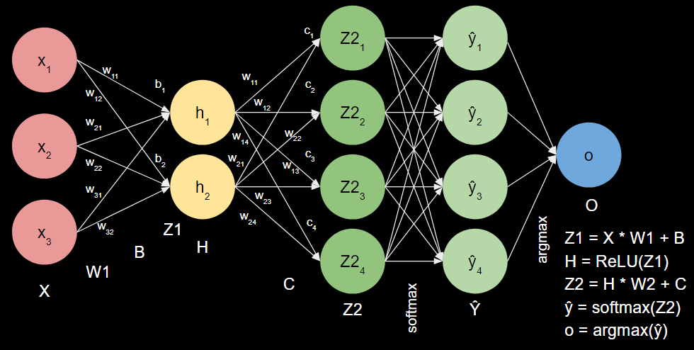
#2: Feedforward Equations for New Neural Network
$X = \begin{bmatrix} x_1 & x_2 & x_3 \end{bmatrix}$
$W1 = \begin{bmatrix} w_{11} & w_{21} & w_{31}\\ w_{12} & w_{22} & w_{32}\\ \end{bmatrix}$
$B = \begin{bmatrix} b_1 & b_2 & b_3 & b_4 \end{bmatrix}$
$Z1 = X * W1.T + B = \begin{bmatrix} z_1\\ z_2 \end{bmatrix}$
$H = ReLU(Z1) = \begin{bmatrix} h_1\\ h_2\\ \end{bmatrix} = \begin{bmatrix} ReLU(z_1)\\ ReLU(z_2)\\ \end{bmatrix}$
$W2 = \begin{bmatrix} w_{11} & w_{21}\\ w_{12} & w_{22}\\ w_{13} & w_{23}\\ w_{14} & w_{24}\\ \end{bmatrix}$
$Z2 = H * W2.T + C = \begin{bmatrix} Z2_1\\ Z2_2\\ Z2_3\\ Z2_4\\ \end{bmatrix}$
$\hat{y} = softmax(Z2) = \begin{bmatrix} \hat{y}_1\\ \hat{y}_2\\ \hat{y}_3\\ \hat{y}_4 \end{bmatrix} = \frac{1}{\sum{e^{\hat{y}}}} \begin{bmatrix} e^{\hat{y}_1}\\ e^{\hat{y}_2}\\ e^{\hat{y}_3}\\ e^{\hat{y}_4} \end{bmatrix}$
$o = argmax(\hat{y})$ (scalar)
$ReLU(z) = max(z, 0)$
$softmax(z) = \frac{e^z}{\sum{e^z}}$
Categorical Cross Entropy:
$L = -\sum{y_i * log(\hat{y}_i)}$
#3 Derivatives of the Loss Function for Each Parameter (W1, B, W2, C)
Before we calculate the derivatives that require the chain rule, let's define each of the partial derivatives that we'll need to use:
Partial derivative of L with respect to $\hat{y}$: $\frac{\partial L}{\partial \hat{y}} = \frac{y}{\hat{y}}$
Partial derivative of $\hat{y}$ with respect to Z2: $\frac{\partial \hat{y}}{\partial Z2} = \begin{bmatrix} \hat{y_1}*(1-\hat{y_1}) & -\hat{y_1}*\hat{y_2} & -\hat{y_1}*\hat{y_3} & -\hat{y_1}*\hat{y_4}\\ -\hat{y_2}*\hat{y_1} & \hat{y_2}*(1-\hat{y_2}) & -\hat{y_2}*\hat{y_3} & -\hat{y_2}*\hat{y_4}\\ -\hat{y_3}*\hat{y_1} & -\hat{y_3}*\hat{y_2} & \hat{y_3}*(1-\hat{y_3}) & -\hat{y_3}*\hat{y_4}\\ -\hat{y_4}*\hat{y_1} & -\hat{y_4}*\hat{y_2} & -\hat{y_4}*\hat{y_3} & \hat{y_4}*(1-\hat{y_4})\\ \end{bmatrix}$
Partial derivative of Z2 with respect to C: $\frac{\partial Z2}{\partial C} = 1$
Partial derivative of Z2 with respect to W2: $\frac{\partial Z2}{\partial W2} = H$
Partial derivative of Z2 with respect to H: $\frac{\partial Z2}{\partial W2} = W2$
Partial derivative of H with respect to Z1: $\frac{\partial H}{\partial Z1} = \begin{cases} 0 \quad if z <= 0\\ 1 \quad if z > 0\\ \end{cases}$
Partial derivative of Z1 with respect to B: $\frac{\partial Z1}{\partial B} = 1$
Partial derivative of Z1 with respect to W1: $\frac{\partial Z1}{\partial W1} = X$
Partial derivative of Z1 with respect to X: $\frac{\partial Z1}{\partial W1} = W1$
Okay, now we're ready to find the partial derivatives of the loss function with respect to each parameter:
Partial derivative of L with respect to C: $\frac{\partial L}{\partial C}\\ \quad = \frac{\partial L}{\partial \hat{y}} * \frac{\partial \hat{y}}{\partial Z2} * \frac{\partial Z2}{\partial C}\\ \quad = \frac{y}{\hat{y}} * \begin{bmatrix} \hat{y_1}*(1-\hat{y_1}) & -\hat{y_1}*\hat{y_2} & -\hat{y_1}*\hat{y_3} & -\hat{y_1}*\hat{y_4}\\ -\hat{y_2}*\hat{y_1} & \hat{y_2}*(1-\hat{y_2}) & -\hat{y_2}*\hat{y_3} & -\hat{y_2}*\hat{y_4}\\ -\hat{y_3}*\hat{y_1} & -\hat{y_3}*\hat{y_2} & \hat{y_3}*(1-\hat{y_3}) & -\hat{y_3}*\hat{y_4}\\ -\hat{y_4}*\hat{y_1} & -\hat{y_4}*\hat{y_2} & -\hat{y_4}*\hat{y_3} & \hat{y_4}*(1-\hat{y_4})\\ \end{bmatrix} * 1 $
Partial derivative of L with respect to W2: $\frac{\partial L}{\partial W2}\\\ \quad = \frac{\partial L}{\partial \hat{y}} * \frac{\partial \hat{y}}{\partial Z2} * \frac{\partial Z2}{\partial W2}\\ \quad = \frac{y}{\hat{y}} * \begin{bmatrix} \hat{y_1}*(1-\hat{y_1}) & -\hat{y_1}*\hat{y_2} & -\hat{y_1}*\hat{y_3} & -\hat{y_1}*\hat{y_4}\\ -\hat{y_2}*\hat{y_1} & \hat{y_2}*(1-\hat{y_2}) & -\hat{y_2}*\hat{y_3} & -\hat{y_2}*\hat{y_4}\\ -\hat{y_3}*\hat{y_1} & -\hat{y_3}*\hat{y_2} & \hat{y_3}*(1-\hat{y_3}) & -\hat{y_3}*\hat{y_4}\\ -\hat{y_4}*\hat{y_1} & -\hat{y_4}*\hat{y_2} & -\hat{y_4}*\hat{y_3} & \hat{y_4}*(1-\hat{y_4})\\ \end{bmatrix} * H \\ \quad = \frac{\partial L}{\partial C} * H $
Partial derivative of L with respect to B: $\frac{\partial L}{\partial B}\\ \quad = \frac{\partial L}{\partial \hat{y}} * \frac{\partial \hat{y}}{\partial Z2} * \frac{\partial Z2}{\partial H} * \frac{\partial H}{\partial Z1} * \frac{\partial Z1}{\partial B}\\ \quad = \frac{y}{\hat{y}} * \begin{bmatrix} \hat{y_1}*(1-\hat{y_1}) & -\hat{y_1}*\hat{y_2} & -\hat{y_1}*\hat{y_3} & -\hat{y_1}*\hat{y_4}\\ -\hat{y_2}*\hat{y_1} & \hat{y_2}*(1-\hat{y_2}) & -\hat{y_2}*\hat{y_3} & -\hat{y_2}*\hat{y_4}\\ -\hat{y_3}*\hat{y_1} & -\hat{y_3}*\hat{y_2} & \hat{y_3}*(1-\hat{y_3}) & -\hat{y_3}*\hat{y_4}\\ -\hat{y_4}*\hat{y_1} & -\hat{y_4}*\hat{y_2} & -\hat{y_4}*\hat{y_3} & \hat{y_4}*(1-\hat{y_4})\\ \end{bmatrix} * W2 * \begin{cases} 0 \quad if z <= 0\\ 1 \quad if z > 0\\ \end{cases} * 1\\ \quad = \frac{\partial L}{\partial C} * W2 * \begin{cases} 0 \quad if z <= 0\\ 1 \quad if z > 0\\ \end{cases} $
Partial derivative of L with respect to W1: $\frac{\partial L}{\partial W1}\\ \quad = \frac{\partial L}{\partial \hat{y}} * \frac{\partial \hat{y}}{\partial Z2} * \frac{\partial Z2}{\partial H} * \frac{\partial H}{\partial Z1} * \frac{\partial Z1}{\partial W1}\\ \quad = \frac{y}{\hat{y}} * \begin{bmatrix} \hat{y_1}*(1-\hat{y_1}) & -\hat{y_1}*\hat{y_2} & -\hat{y_1}*\hat{y_3} & -\hat{y_1}*\hat{y_4}\\ -\hat{y_2}*\hat{y_1} & \hat{y_2}*(1-\hat{y_2}) & -\hat{y_2}*\hat{y_3} & -\hat{y_2}*\hat{y_4}\\ -\hat{y_3}*\hat{y_1} & -\hat{y_3}*\hat{y_2} & \hat{y_3}*(1-\hat{y_3}) & -\hat{y_3}*\hat{y_4}\\ -\hat{y_4}*\hat{y_1} & -\hat{y_4}*\hat{y_2} & -\hat{y_4}*\hat{y_3} & \hat{y_4}*(1-\hat{y_4})\\ \end{bmatrix} * W2 * \begin{cases} 0 \quad if z <= 0\\ 1 \quad if z > 0\\ \end{cases} * X\\ \quad = \frac{\partial L}{\partial C} * W2 * \begin{cases} 0 \quad if z <= 0\\ 1 \quad if z > 0\\ \end{cases} * X \\ \quad = \frac{\partial L}{\partial B} * X $
#4: Test Calculation of Softmax
Assume $Z2 = \begin{bmatrix} 1.1 \\ 2.2 \\ 0.2 \\ -1.7 \end{bmatrix}$, let's calculate $\hat{y}$.
$\hat{y} = softmax(Z2)\\ \quad = \frac{1}{\sum{e^{Z2_i}}} \begin{bmatrix} e^{1.1} \\ e^{2.2} \\ e^{0.2} \\ e^{-1.7} \\ \end{bmatrix}\\ \quad = \frac{1}{e^{1.1} + e^{2.2} + e^{0.2} + e^{-1.7}} \begin{bmatrix} e^{1.1} \\ e^{2.2} \\ e^{0.2} \\ e^{-1.7} \\ \end{bmatrix}\\ \quad = \frac{1}{13.43} \begin{bmatrix} 3.004 \\ 9.025 \\ 1.221 \\ 0.1827 \end{bmatrix}\\ \quad = \begin{bmatrix} 0.224 \\ 0.672 \\ 0.091 \\ 0.014 \end{bmatrix}\\ $
#5 Write out the Derivative for Softmax when $i = j$ and when $i \neq j$
A reminder that softmax is defined as follows: $\hat{y_i} = \frac{e^{Z_i}}{\sum{e^{Z_j}}}$
Another reminder on the quotient rule. If $f(x) = \frac{u(x)}{v(x)}$, then $f'(x) = \frac{u'(x)v(x) - u(x)v'(x)}{v(x)^2}$
Here we have $u(x) = e^{Z_i}$ and $v(x) = \sum{e^{Z_j}}$
First, let's calculate the derivative when $i \neq j$.
Now, $u'(z_j) = 0$ and $v'(x) = e^{Z_j}$
$\frac{\partial \hat{y}}{\partial Z_j } = \frac{u'(x)v(x) - u(x)v'(x)}{v(x)^2}\\ \quad = \frac{0 * \sum{e^{Z_j}} - e^{Z_i} * e^{Z_j}}{(\sum{e^{Z_j}})^2}\\ \quad = -\frac{e^{Z_i}}{\sum{e^{Z_j}}}*\frac{e^{Z_j}}{\sum{e^{Z_j}}}\\ \quad = -\hat{y_i}\hat{y_j} $
Now, let's calculate the derivative when $i = j$.
Since $i = j$, $z_i = z_j$,
now $u'(z_i) = e^{Z_i}$ and $v'(x) = e^{Z_j} = e^{Z_i}$
$\frac{\partial \hat{y}}{\partial Z_j } = \frac{u'(x)v(x) - u(x)v'(x)}{v(x)^2}\\ \quad = \frac{e^{Z_i} * \sum{e^{Z_j}} - e^{Z_i} * e^{Z_i}}{(\sum{e^{Z_j}})^2}\\ \quad = \frac{e^{Z_i}}{\sum{e^{Z_j}}}*\frac{\sum{e^{Z_j}}-e^{Z_i}}{\sum{e^{Z_j}}}\\ \quad = \frac{e^{Z_i}}{\sum{e^{Z_j}}}(1-\frac{e^{Z_i}}{\sum{e^{Z_j}}})\\ \quad = \hat{y_i}(1 - \hat{y_j})\\ $
Written in matrix form as the Jacobian, we have:
$\frac{\partial \hat{y}}{\partial Z } =
\begin{bmatrix}
\hat{y_1}(1-\hat{y_1}) & -\hat{y_1}\hat{y_2} & -\hat{y_1}\hat{y_3} & -\hat{y_1}\hat{y_4}\\
-\hat{y_2}\hat{y_1} & \hat{y_2}(1-\hat{y_2}) & -\hat{y_2}\hat{y_3} & -\hat{y_2}\hat{y_4}\\
-\hat{y_3}\hat{y_1} & -\hat{y_3}\hat{y_2} & \hat{y_3}(1-\hat{y_3}) & -\hat{y_3}\hat{y_4}\\
-\hat{y_4}\hat{y_1} & -\hat{y_4}\hat{y_2} & -\hat{y_4}\hat{y_3} & \hat{y_4}(1-\hat{y_4})\\
\end{bmatrix}
$
#6: Partial Derivative of Loss with Respect to $Z2$
$\frac{\partial L}{\partial Z2} = \frac{\partial L}{\partial \hat{y}} * \frac{\partial \hat{y}}{\partial Z2}\\ \quad = -\sum_{i} \frac{y_i}{\hat{y_i}} * \begin{cases} \hat{y_i}(1 - \hat{y_j}) \quad if i = j\\ \hat{y_i}\hat{y_j} \quad\quad if i \neq j\\ \end{cases} \\ \quad = \hat{y}_i - y_i $
#7: Neural Network with Softmax, Categorical Cross Entropy, and ReLU Activation Coded
# create a function to one-hot-encode categorical data
def one_hot_encode(y):
    y_values = set(y)
    y_length = len(y_values)
    # convert values in y to integers
    for i, item in enumerate(y_values):
        y[y == item] = i

    # create new y array with one hot encoding
    y_new = np.zeros((len(y), y_length))
    for i, item in enumerate(y):
        y_new[i, item] = 1
    return y_new.astype(int)

df2 = pd.read_csv('A2_Pt2_Data_ILG.csv')
x2, y2 = get_xy(df2)
x2 = normalize(x2)
y2 = one_hot_encode(y2)

print('The data is: \n', df2)
print('\nX normalized is: \n', x2)
print('\nY one hot encoded is: \n', y2)
The data is:
     experience  skill  athleticism  label
0            5      8            5      3
1            4      4            3      3
2            5      6            4      3
3            5      4            5      3
4            2      5            5      2
5            4      8            5      2
6            3      7            3      2
7            5      8            2      2
8            2      3            4      1
9            0      2            3      1
10           1      2            1      1
11           0      2            3      1
12           2      1            0      0
13           1      0            1      0
14           1      1            0      0
15           0      0            0      0
16           0      0            1      0

X normalized is:
 [[1.    1.    1.   ]
 [0.6   0.8   0.5  ]
 [0.8   1.    0.75 ]
 [1.    1.    0.5  ]
 [1.    0.4   0.625]
 [1.    0.8   1.   ]
 [0.6   0.6   0.875]
 [0.4   1.    1.   ]
 [0.8   0.4   0.375]
 [0.6   0.    0.25 ]
 [0.2   0.2   0.25 ]
 [0.6   0.    0.25 ]
 [0.    0.4   0.125]
 [0.2   0.2   0.   ]
 [0.    0.2   0.125]
 [0.    0.    0.   ]
 [0.2   0.    0.   ]]

Y one hot encoded is:
 [[0 0 0 1]
 [0 0 0 1]
 [0 0 0 1]
 [0 0 0 1]
 [0 0 1 0]
 [0 0 1 0]
 [0 0 1 0]
 [0 0 1 0]
 [0 1 0 0]
 [0 1 0 0]
 [0 1 0 0]
 [0 1 0 0]
 [1 0 0 0]
 [1 0 0 0]
 [1 0 0 0]
 [1 0 0 0]
 [1 0 0 0]]
import pandas as pd
import numpy as np
import matplotlib.pyplot as plt
from sklearn.metrics import confusion_matrix, ConfusionMatrixDisplay, accuracy_score

# activation function
def relu(z):
    return np.maximum(0, z)
def relu_derivative(z):
    return np.where(z > 0, 1, 0)

# loss function
def cce(y, y_hat):
    return -np.sum(y*np.log(y_hat))

# output layer activation function
def softmax(z):
    return np.exp(z)/np.sum(np.exp(z), axis=1).reshape(-1, 1)


#2: Code the feedforward function
class NeuralNetworkCCE():
    # assumes one hidden layer
    # assumes one-hot-encoded y
    # assumes softmax activation on output layer
    # assumes cross-entropy loss

    def __init__(self, LR=0.1, epochs=10, activation='relu', input_layer_dim=3, hidden_layer_dim=2, output_layer_dim=4):
        self.LR = LR
        self.epochs = epochs
        # shape parameters
        self.hidden_layer_dim = hidden_layer_dim
        self.output_layer_dim = output_layer_dim
        self.input_layer_dim = input_layer_dim

        if activation == 'relu':
            self.activation = relu
            self.activation_derivative = relu_derivative
        elif activation == 'sigmoid':
            self.activation = sigmoid
            self.activation_derivative = sigmoid_derivative

        # initialize with weights as ones and biases as zeros
        self.w1 = np.ones((self.hidden_layer_dim, self.input_layer_dim))
        self.b = np.zeros((1, self.hidden_layer_dim))
        self.w2 = np.ones((self.output_layer_dim, self.hidden_layer_dim))
        self.c = np.zeros((1, self.output_layer_dim))

    def randomize_weights(self):
        np.random.seed(44)
        self.w1 = np.random.rand(self.hidden_layer_dim, self.input_layer_dim)
        self.b = np.random.rand(1, self.hidden_layer_dim)
        self.w2 = np.random.rand(self.output_layer_dim, self.hidden_layer_dim)
        self.c = np.random.rand(1, self.output_layer_dim)

    def feed_forward(self, x):
        self.z1 = (x @ self.w1.T + self.b).astype(float)
        self.h = self.activation(self.z1).astype(float)
        self.z2 = (self.h @ self.w2.T + self.c).astype(float)
        self.y_hat = softmax(self.z2).astype(float)
        self.output = np.argmax(self.y_hat, axis=1).reshape(-1, 1)
        return

    def calculate_loss(self, y):
        self.loss = cce(y, self.y_hat).astype(float)
        return

    def print_params(self):
        print('\nW1 is: \n', self.w1) # shape is (2x3)
        print('\nB is: \n', self.b) # shape is (1x2)
        print('\nZ1 is: \n', self.z1) # shape is (17x2)
        print('\nH is: \n', self.h) # shape is (17x2)
        print('\nW2 is: \n', self.w2) # shape is (4x2)
        print('\nZ2 is: \n', self.z2) # shape is (17x4)
        print('\nC is: \n', self.c) # shape is (1x4)
        print('\ny^ is: \n', self.y_hat) # shape is (17x4)
        print('\noutput is: \n', self.output) # shape is (17x1)
        print('\nL is: \n', self.loss) # shape is (1x1)


    def backpropogate(self, x, y):
        self.dLdC = (self.y_hat - y).astype(float) # shape is (17x4)
        self.dLdW2 = (self.dLdC.T @ self.h).astype(float) # (4x17)*(17x2) = (4x2)
        self.dLdB = (self.dLdC @ self.w2 * self.activation_derivative(self.z1)).astype(float) # (17x4) @ (4x2) * (17x2) = (17x2)
        self.dLdW1 = (self.dLdB.T @ x).astype(float) # (2x17)*(17x3) = (2x3)

    def print_derivatives(self):
        print('\ndLdC is: \n', self.dLdC) # shape is (17x4)
        print('\ndLdW2 is: \n', self.dLdW2) # shape is (4x2)
        print('\ndLdB is: \n', self.dLdB) # shape is (17x2)
        print('\ndLdW1 is \n', self.dLdW1) # shape is (2x3)

    def update_params(self):
        self.c = (self.c - self.LR * self.dLdC.mean(axis=0)).astype(float) # (1x4)-LR*(17x4).mean = (1x4)
        self.w2 = (self.w2 - self.LR * self.dLdW2).astype(float) # (4x2)-LR*(4x2).mean = (4x2)
        self.b = (self.b - self.LR * self.dLdB.mean(axis=0)).astype(float) # (1x2)-LR*(17x2).mean = (1x2)
        self.w1 = (self.w1 - self.LR * self.dLdW1).astype(float) # (2x3)-LR*(2x3) = (2x3)
        return

    def train(self, x, y, verbose=False, plot=True):
        if verbose:
            print('Preparing to train Neural Network...')
            print('X is: \n', x)
            print('\ny is: \n', y)
        self.randomize_weights()
        self.loss_by_epoch = []
        for e in range(self.epochs):
            if verbose:
                print('###############################################################\nNow running epoch', e+1, 'of', self.epochs, 'total epochs.')
                print('Feeding forward...')
            self.feed_forward(x)
            if verbose:
                print('Calculating loss...')
            self.calculate_loss(y)
            if verbose:
                print('The parameters are: ')
                self.print_params()
                print('\nPerforming backpropogation...')
            self.backpropogate(x, y)
            self.update_params()
            if verbose:
                print('The derivatives are: ')
                self.print_derivatives()
                print('\nFinished epoch', e+1, 'with loss', self.loss)
            self.loss_by_epoch.append(self.loss)
        if verbose:
            print('Training complete! Loss by epoch is: \n', self.loss_by_epoch)
        if plot:
            y = self.loss_by_epoch
            x = range(self.epochs)
            plt.plot(x, y)
            plt.xlabel('Epoch')
            plt.ylabel('Loss')
            plt.title('Loss by Epoch')
            plt.show()

    # multilabel confusion matrix
    def plot_confusion_matrix(self, y):
        y_pred = self.output
        y = np.argmax(self.y_hat, axis=1).reshape(-1, 1)
        self.cm = confusion_matrix(y, y_pred)
        classes = ['0: Bad', '1: Okay', '2: Good', '3: Great']
        display = ConfusionMatrixDisplay(self.cm, display_labels=classes)
        display.ax_.set_title('Confusion Matrix for Player Ability Prediction')
        display.plot()
        # calculate accuracy
        self.accuracy = accuracy_score(y, y_pred)
        print('Accuracy is: ', self.accuracy)

    def predict(self, x, y):
        self.feed_forward(x)
        self.plot_confusion_matrix(y)
# test code with verbose mode
nn4 = NeuralNetworkCCE(
    LR=0.001,
    epochs=2,
    activation='relu',
    input_layer_dim=3,
    hidden_layer_dim=2,
    output_layer_dim=4
)
nn4.train(x2, y2, verbose=True, plot=False)
Preparing to train Neural Network...
X is:
 [[1.    1.    1.   ]
 [0.6   0.8   0.5  ]
 [0.8   1.    0.75 ]
 [1.    1.    0.5  ]
 [1.    0.4   0.625]
 [1.    0.8   1.   ]
 [0.6   0.6   0.875]
 [0.4   1.    1.   ]
 [0.8   0.4   0.375]
 [0.6   0.    0.25 ]
 [0.2   0.2   0.25 ]
 [0.6   0.    0.25 ]
 [0.    0.4   0.125]
 [0.2   0.2   0.   ]
 [0.    0.2   0.125]
 [0.    0.    0.   ]
 [0.2   0.    0.   ]]

y is:
 [[0 0 0 1]
 [0 0 0 1]
 [0 0 0 1]
 [0 0 0 1]
 [0 0 1 0]
 [0 0 1 0]
 [0 0 1 0]
 [0 0 1 0]
 [0 1 0 0]
 [0 1 0 0]
 [0 1 0 0]
 [0 1 0 0]
 [1 0 0 0]
 [1 0 0 0]
 [1 0 0 0]
 [1 0 0 0]
 [1 0 0 0]]
###############################################################
Now running epoch 1 of 2 total epochs.
Feeding forward...
Calculating loss...
The parameters are:

W1 is:
 [[0.834842 0.104796 0.74464 ]
 [0.360501 0.359311 0.609238]]

B is:
 [[0.39378  0.409073]]

Z1 is:
 [[2.078058 1.738123]
 [1.350842 1.217441]
 [1.72493  1.513713]
 [1.705738 1.433503]
 [1.73594  1.294072]
 [2.057099 1.66626 ]
 [1.609123 1.374043]
 [1.577153 1.521822]
 [1.382812 1.069662]
 [1.080845 0.777683]
 [0.767867 0.705345]
 [1.080845 0.777683]
 [0.528778 0.628952]
 [0.581707 0.553035]
 [0.507819 0.55709 ]
 [0.39378  0.409073]
 [0.560748 0.481173]]

H is:
 [[2.078058 1.738123]
 [1.350842 1.217441]
 [1.72493  1.513713]
 [1.705738 1.433503]
 [1.73594  1.294072]
 [2.057099 1.66626 ]
 [1.609123 1.374043]
 [1.577153 1.521822]
 [1.382812 1.069662]
 [1.080845 0.777683]
 [0.767867 0.705345]
 [1.080845 0.777683]
 [0.528778 0.628952]
 [0.581707 0.553035]
 [0.507819 0.55709 ]
 [0.39378  0.409073]
 [0.560748 0.481173]]

W2 is:
 [[0.509902 0.710148]
 [0.960526 0.456621]
 [0.427652 0.113464]
 [0.217899 0.957472]]

Z2 is:
 [[3.237282 3.671517 1.732309 2.330835]
 [2.496712 2.735253 1.362236 1.673837]
 [2.897857 3.229858 1.555831 2.039023]
 [2.83111  3.174798 1.538523 1.958043]
 [2.747493 3.140141 1.535618 1.831122]
 [3.175562 3.618572 1.715192 2.257462]
 [2.73962  3.054846 1.490458 1.880059]
 [2.828264 3.091617 1.493554 2.014587]
 [2.408068 2.698482 1.35914  1.539309]
 [2.046746 2.275111 1.196874 1.193949]
 [1.835787 1.941456 1.054821 1.05649 ]
 [2.046746 2.275111 1.196874 1.193949]
 [1.659625 1.676922 0.943906 0.931249]
 [1.632701 1.693097 0.957928 0.870094]
 [1.597905 1.623976 0.92679  0.857876]
 [1.434642 1.446851 0.861226 0.691305]
 [1.570981 1.640151 0.940811 0.796721]]

C is:
 [[0.943351 0.881824 0.646411 0.213825]]

y^ is:
 [[0.315481 0.487034 0.070044 0.127441]
 [0.330016 0.418921 0.10613  0.144932]
 [0.32481  0.452705 0.084878 0.137608]
 [0.322335 0.454536 0.0885   0.134629]
 [0.314614 0.46591  0.093641 0.125835]
 [0.313596 0.488391 0.072801 0.125212]
 [0.324606 0.444894 0.093079 0.137421]
 [0.332475 0.432645 0.087519 0.147361]
 [0.321878 0.430345 0.112758 0.135019]
 [0.321519 0.404003 0.13744  0.137038]
 [0.330235 0.367041 0.151236 0.151488]
 [0.321519 0.404003 0.13744  0.137038]
 [0.334562 0.3404   0.163548 0.161491]
 [0.329166 0.349659 0.167635 0.153539]
 [0.331713 0.340475 0.169551 0.15826 ]
 [0.327718 0.331744 0.184701 0.155838]
 [0.326247 0.349612 0.173727 0.150414]]

output is:
 [[1]
 [1]
 [1]
 [1]
 [1]
 [1]
 [1]
 [1]
 [1]
 [1]
 [1]
 [1]
 [1]
 [1]
 [1]
 [1]
 [1]]

L is:
 26.98211399485623

Performing backpropogation...
The derivatives are:

dLdC is:
 [[ 0.315481  0.487034  0.070044 -0.872559]
 [ 0.330016  0.418921  0.10613  -0.855068]
 [ 0.32481   0.452705  0.084878 -0.862392]
 [ 0.322335  0.454536  0.0885   -0.865371]
 [ 0.314614  0.46591  -0.906359  0.125835]
 [ 0.313596  0.488391 -0.927199  0.125212]
 [ 0.324606  0.444894 -0.906921  0.137421]
 [ 0.332475  0.432645 -0.912481  0.147361]
 [ 0.321878 -0.569655  0.112758  0.135019]
 [ 0.321519 -0.595997  0.13744   0.137038]
 [ 0.330235 -0.632959  0.151236  0.151488]
 [ 0.321519 -0.595997  0.13744   0.137038]
 [-0.665438  0.3404    0.163548  0.161491]
 [-0.670834  0.349659  0.167635  0.153539]
 [-0.668287  0.340475  0.169551  0.15826 ]
 [-0.672282  0.331744  0.184701  0.155838]
 [-0.673753  0.349612  0.173727  0.150414]]

dLdW2 is:
 [[ 4.119118  3.1018  ]
 [ 4.66674   4.29809 ]
 [-4.783508 -3.956101]
 [-4.002351 -3.443789]]

dLdB is:
 [[ 0.468498 -0.381075]
 [ 0.429729 -0.381013]
 [ 0.44884  -0.378709]
 [ 0.450237 -0.382071]
 [ 0.247755  0.453811]
 [ 0.259781  0.460393]
 [ 0.234948  0.46234 ]
 [ 0.226983  0.471222]
 [-0.305401  0.110535]
 [-0.319891  0.102986]
 [-0.341901  0.107699]
 [-0.319891  0.102986]
 [ 0.092784 -0.143946]
 [ 0.098943 -0.150699]
 [ 0.093268 -0.148347]
 [ 0.088795 -0.155772]
 [ 0.099333 -0.155095]]

dLdW1 is
 [[ 1.618028  2.271252  1.755612]
 [ 0.257769 -0.199834  0.656478]]

Finished epoch 1 with loss 26.98211399485623
###############################################################
Now running epoch 2 of 2 total epochs.
Feeding forward...
Calculating loss...
The parameters are:

W1 is:
 [[0.833224 0.102525 0.742885]
 [0.360243 0.359511 0.608582]]

B is:
 [[0.393665 0.409073]]

Z1 is:
 [[2.072299 1.737409]
 [1.347061 1.217118]
 [1.719932 1.513214]
 [1.700856 1.433118]
 [1.732202 1.293484]
 [2.051794 1.665506]
 [1.605138 1.373434]
 [1.572364 1.521263]
 [1.379836 1.06929 ]
 [1.07932  0.777364]
 [0.766536 0.705169]
 [1.07932  0.777364]
 [0.527535 0.62895 ]
 [0.580814 0.553024]
 [0.50703  0.557048]
 [0.393665 0.409073]
 [0.56031  0.481122]]

H is:
 [[2.072299 1.737409]
 [1.347061 1.217118]
 [1.719932 1.513214]
 [1.700856 1.433118]
 [1.732202 1.293484]
 [2.051794 1.665506]
 [1.605138 1.373434]
 [1.572364 1.521263]
 [1.379836 1.06929 ]
 [1.07932  0.777364]
 [0.766536 0.705169]
 [1.07932  0.777364]
 [0.527535 0.62895 ]
 [0.580814 0.553024]
 [0.50703  0.557048]
 [0.393665 0.409073]
 [0.56031  0.481122]]

W2 is:
 [[0.505783 0.707046]
 [0.955859 0.452323]
 [0.432435 0.11742 ]
 [0.221901 0.960916]]

Z2 is:
 [[3.219882 3.648346 1.746663 2.343267]
 [2.4852   2.719782 1.371953 1.682381]
 [2.883146 3.210126 1.567963 2.049645]
 [2.816865 3.155662 1.550309 1.968445]
 [2.733992 3.122464 1.547468 1.841225]
 [3.158673 3.596223 1.729353 2.269625]
 [2.726254 3.037173 1.501909 1.889855]
 [2.814198 3.072711 1.505094 2.024633]
 [2.397255 2.684244 1.368768 1.547603]
 [2.038855 2.264948 1.204537 1.200402]
 [1.829608 1.933315 1.0608   1.061621]
 [2.038855 2.264948 1.204537 1.200402]
 [1.654835 1.670388 0.948499 0.935346]
 [1.6281   1.686972 0.962623 0.87421 ]
 [1.593626 1.618265 0.931189 0.861704]
 [1.431662 1.442971 0.86479  0.694357]
 [1.56689  1.63485  0.945313 0.800568]]

C is:
 [[0.94332  0.88165  0.646523 0.213918]]

y^ is:
 [[0.314438 0.482631 0.072065 0.130866]
 [0.328846 0.415787 0.108023 0.147344]
 [0.323653 0.448834 0.086877 0.140636]
 [0.321218 0.450752 0.090519 0.137511]
 [0.313526 0.462365 0.095713 0.128395]
 [0.312556 0.484121 0.074848 0.128475]
 [0.323426 0.441373 0.095071 0.14013 ]
 [0.331224 0.428936 0.089451 0.150389]
 [0.320768 0.427394 0.11469  0.137149]
 [0.320488 0.401793 0.139146 0.138572]
 [0.329295 0.365279 0.15265  0.152775]
 [0.320488 0.401793 0.139146 0.138572]
 [0.333765 0.338996 0.164696 0.162544]
 [0.328385 0.348299 0.1688   0.154516]
 [0.330959 0.339215 0.17064  0.159186]
 [0.32711  0.330831 0.185569 0.15649 ]
 [0.325506 0.348396 0.174828 0.151269]]

output is:
 [[1]
 [1]
 [1]
 [1]
 [1]
 [1]
 [1]
 [1]
 [1]
 [1]
 [1]
 [1]
 [1]
 [1]
 [1]
 [1]
 [1]]

L is:
 26.83734192204232

Performing backpropogation...
The derivatives are:

dLdC is:
 [[ 0.314438  0.482631  0.072065 -0.869134]
 [ 0.328846  0.415787  0.108023 -0.852656]
 [ 0.323653  0.448834  0.086877 -0.859364]
 [ 0.321218  0.450752  0.090519 -0.862489]
 [ 0.313526  0.462365 -0.904287  0.128395]
 [ 0.312556  0.484121 -0.925152  0.128475]
 [ 0.323426  0.441373 -0.904929  0.14013 ]
 [ 0.331224  0.428936 -0.910549  0.150389]
 [ 0.320768 -0.572606  0.11469   0.137149]
 [ 0.320488 -0.598207  0.139146  0.138572]
 [ 0.329295 -0.634721  0.15265   0.152775]
 [ 0.320488 -0.598207  0.139146  0.138572]
 [-0.666235  0.338996  0.164696  0.162544]
 [-0.671615  0.348299  0.1688    0.154516]
 [-0.669041  0.339215  0.17064   0.159186]
 [-0.67289   0.330831  0.185569  0.15649 ]
 [-0.674494  0.348396  0.174828  0.151269]]

dLdW2 is:
 [[ 4.085186  3.081406]
 [ 4.586622  4.240666]
 [-4.732556 -3.922069]
 [-3.939253 -3.400002]]

dLdB is:
 [[ 0.458666 -0.386076]
 [ 0.421266 -0.386067]
 [ 0.439595 -0.38372 ]
 [ 0.441079 -0.387149]
 [ 0.237978  0.448012]
 [ 0.249278  0.454793]
 [ 0.225246  0.456717]
 [ 0.217148  0.465803]
 [-0.305063  0.11305 ]
 [-0.318783  0.105512]
 [-0.34024   0.110457]
 [-0.318783  0.105512]
 [ 0.094351 -0.142194]
 [ 0.100516 -0.149021]
 [ 0.094966 -0.146607]
 [ 0.090863 -0.153958]
 [ 0.101039 -0.153425]]

dLdW1 is
 [[ 1.559117  2.210026  1.696602]
 [ 0.229971 -0.231618  0.626421]]

Finished epoch 2 with loss 26.83734192204232
Training complete! Loss by epoch is:
 [26.98211399485623, 26.83734192204232]
# test the code with 1000 epochs and verbose mode off, plot on
nn5 = NeuralNetworkCCE(
    LR=0.1,
    epochs=1000,
    activation='relu',
    input_layer_dim=3,
    hidden_layer_dim=2,
    output_layer_dim=4
)
nn5.train(x2, y2, verbose=False, plot=True)
nn5.plot_confusion_matrix(y2)

Accuracy is: 1.0

# export to HTML for webpage
import os

# os.system('jupyter nbconvert --to html mod1.ipynb')
os.system('jupyter nbconvert --to html mod2.ipynb --HTMLExporter.theme=dark')