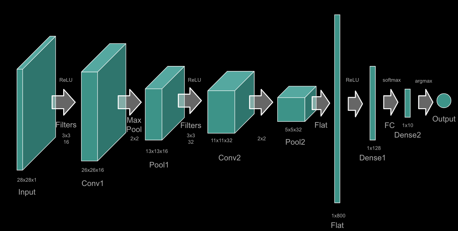
Here, I build a simple convolutional neural network (CNN) to classify the MNIST digits dataset. I use the Keras API with the TensorFlow backend. I use the sequential model with two convolutional layers and two max pooling layers. I then flatten the output of the second max pooling layer and use two dense layers to classify the digits. I use the Adam optimizer and the sparse categorial cross entropy loss function.
In addition, I illustrate the raw data as both a matrix and as an image. I also illustrate the dataset sizes. Finally, I illustrate the accuracy and loss of the model as a function of the epoch number and a confusion matrix of the results.
Below is a diagram of the CNN model.

# import libraries
import numpy as np
import tensorflow as tf
from tensorflow import keras
from keras import layers, models
import matplotlib.pyplot as plt
from sklearn.metrics import confusion_matrix
# import mnist data
data = tf.keras.datasets.mnist.load_data(path="mnist.npz")
# split the data into test/train
x_train, y_train = data[0]
x_test, y_test = data[1]
# print the first value of x_train as a matrix
print('The first value of x_train as a matrix:')
print(x_train[0])
The first value of x_train as a matrix:
[[ 0 0 0 0 0 0 0 0 0 0 0 0 0 0 0 0 0 0
0 0 0 0 0 0 0 0 0 0]
[ 0 0 0 0 0 0 0 0 0 0 0 0 0 0 0 0 0 0
0 0 0 0 0 0 0 0 0 0]
[ 0 0 0 0 0 0 0 0 0 0 0 0 0 0 0 0 0 0
0 0 0 0 0 0 0 0 0 0]
[ 0 0 0 0 0 0 0 0 0 0 0 0 0 0 0 0 0 0
0 0 0 0 0 0 0 0 0 0]
[ 0 0 0 0 0 0 0 0 0 0 0 0 0 0 0 0 0 0
0 0 0 0 0 0 0 0 0 0]
[ 0 0 0 0 0 0 0 0 0 0 0 0 3 18 18 18 126 136
175 26 166 255 247 127 0 0 0 0]
[ 0 0 0 0 0 0 0 0 30 36 94 154 170 253 253 253 253 253
225 172 253 242 195 64 0 0 0 0]
[ 0 0 0 0 0 0 0 49 238 253 253 253 253 253 253 253 253 251
93 82 82 56 39 0 0 0 0 0]
[ 0 0 0 0 0 0 0 18 219 253 253 253 253 253 198 182 247 241
0 0 0 0 0 0 0 0 0 0]
[ 0 0 0 0 0 0 0 0 80 156 107 253 253 205 11 0 43 154
0 0 0 0 0 0 0 0 0 0]
[ 0 0 0 0 0 0 0 0 0 14 1 154 253 90 0 0 0 0
0 0 0 0 0 0 0 0 0 0]
[ 0 0 0 0 0 0 0 0 0 0 0 139 253 190 2 0 0 0
0 0 0 0 0 0 0 0 0 0]
[ 0 0 0 0 0 0 0 0 0 0 0 11 190 253 70 0 0 0
0 0 0 0 0 0 0 0 0 0]
[ 0 0 0 0 0 0 0 0 0 0 0 0 35 241 225 160 108 1
0 0 0 0 0 0 0 0 0 0]
[ 0 0 0 0 0 0 0 0 0 0 0 0 0 81 240 253 253 119
25 0 0 0 0 0 0 0 0 0]
[ 0 0 0 0 0 0 0 0 0 0 0 0 0 0 45 186 253 253
150 27 0 0 0 0 0 0 0 0]
[ 0 0 0 0 0 0 0 0 0 0 0 0 0 0 0 16 93 252
253 187 0 0 0 0 0 0 0 0]
[ 0 0 0 0 0 0 0 0 0 0 0 0 0 0 0 0 0 249
253 249 64 0 0 0 0 0 0 0]
[ 0 0 0 0 0 0 0 0 0 0 0 0 0 0 46 130 183 253
253 207 2 0 0 0 0 0 0 0]
[ 0 0 0 0 0 0 0 0 0 0 0 0 39 148 229 253 253 253
250 182 0 0 0 0 0 0 0 0]
[ 0 0 0 0 0 0 0 0 0 0 24 114 221 253 253 253 253 201
78 0 0 0 0 0 0 0 0 0]
[ 0 0 0 0 0 0 0 0 23 66 213 253 253 253 253 198 81 2
0 0 0 0 0 0 0 0 0 0]
[ 0 0 0 0 0 0 18 171 219 253 253 253 253 195 80 9 0 0
0 0 0 0 0 0 0 0 0 0]
[ 0 0 0 0 55 172 226 253 253 253 253 244 133 11 0 0 0 0
0 0 0 0 0 0 0 0 0 0]
[ 0 0 0 0 136 253 253 253 212 135 132 16 0 0 0 0 0 0
0 0 0 0 0 0 0 0 0 0]
[ 0 0 0 0 0 0 0 0 0 0 0 0 0 0 0 0 0 0
0 0 0 0 0 0 0 0 0 0]
[ 0 0 0 0 0 0 0 0 0 0 0 0 0 0 0 0 0 0
0 0 0 0 0 0 0 0 0 0]
[ 0 0 0 0 0 0 0 0 0 0 0 0 0 0 0 0 0 0
0 0 0 0 0 0 0 0 0 0]]
# print the first value of x_train as an image
print('The first value of x_train as an image:')
plt.imshow(x_train[0], cmap=plt.cm.binary)
plt.show()
The first value of x_train as an image:
# normalize the data
x_train = x_train / 255.0
x_test = x_test / 255.0
# clear the session
tf.keras.backend.clear_session()
# initialize the model
cnn = keras.Sequential()
# add layers
# first convolutional layer
cnn.add(layers.Conv2D(
filters=16,
kernel_size=(3, 3),
activation='relu',
input_shape=(28, 28, 1),
padding='valid' # don't add padding, default value
))
# first pooling layer
cnn.add(layers.MaxPooling2D(
pool_size=(2, 2)
))
# second convolutional layer
cnn.add(layers.Conv2D(
filters=32,
kernel_size=(3, 3),
activation='relu',
padding='valid' # don't add padding, default value
))
# second pooling layer
cnn.add(layers.MaxPooling2D(
pool_size=(2, 2)
))
# flatten the data
cnn.add(layers.Flatten())
# add a dense layer
cnn.add(layers.Dense(
units=128,
activation='relu'
))
# add an output layer
cnn.add(layers.Dense(
units=10,
activation='softmax'
))
# compile the model
cnn.compile(
loss = 'sparse_categorical_crossentropy',
optimizer = 'adam',
metrics = ['accuracy']
)
cnn.summary()
Model: "sequential"
_________________________________________________________________
Layer (type) Output Shape Param #
=================================================================
conv2d (Conv2D) (None, 26, 26, 16) 160
max_pooling2d (MaxPooling2 (None, 13, 13, 16) 0
D)
conv2d_1 (Conv2D) (None, 11, 11, 32) 4640
max_pooling2d_1 (MaxPoolin (None, 5, 5, 32) 0
g2D)
flatten (Flatten) (None, 800) 0
dense (Dense) (None, 128) 102528
dense_1 (Dense) (None, 10) 1290
=================================================================
Total params: 108618 (424.29 KB)
Trainable params: 108618 (424.29 KB)
Non-trainable params: 0 (0.00 Byte)
_________________________________________________________________
# train the model
history = cnn.fit(
x_train,
y_train,
epochs=10,
batch_size=128,
validation_data=(x_test, y_test),
verbose=1
)
Epoch 1/10 469/469 [==============================] - 15s 30ms/step - loss: 0.2679 - accuracy: 0.9272 - val_loss: 0.0659 - val_accuracy: 0.9803 Epoch 2/10 469/469 [==============================] - 15s 31ms/step - loss: 0.0630 - accuracy: 0.9814 - val_loss: 0.0438 - val_accuracy: 0.9849 Epoch 3/10 469/469 [==============================] - 17s 37ms/step - loss: 0.0433 - accuracy: 0.9871 - val_loss: 0.0346 - val_accuracy: 0.9882 Epoch 4/10 469/469 [==============================] - 16s 33ms/step - loss: 0.0357 - accuracy: 0.9888 - val_loss: 0.0296 - val_accuracy: 0.9907 Epoch 5/10 469/469 [==============================] - 14s 30ms/step - loss: 0.0288 - accuracy: 0.9909 - val_loss: 0.0330 - val_accuracy: 0.9889 Epoch 6/10 469/469 [==============================] - 13s 27ms/step - loss: 0.0243 - accuracy: 0.9926 - val_loss: 0.0312 - val_accuracy: 0.9897 Epoch 7/10 469/469 [==============================] - 14s 30ms/step - loss: 0.0197 - accuracy: 0.9938 - val_loss: 0.0306 - val_accuracy: 0.9902 Epoch 8/10 469/469 [==============================] - 15s 31ms/step - loss: 0.0152 - accuracy: 0.9952 - val_loss: 0.0329 - val_accuracy: 0.9903 Epoch 9/10 469/469 [==============================] - 14s 30ms/step - loss: 0.0132 - accuracy: 0.9955 - val_loss: 0.0268 - val_accuracy: 0.9904 Epoch 10/10 469/469 [==============================] - 14s 29ms/step - loss: 0.0118 - accuracy: 0.9961 - val_loss: 0.0328 - val_accuracy: 0.9903
# evaluate the model
test_loss, test_accuracy = cnn.evaluate(x_test, y_test, verbose=1)
predictions = cnn.predict(x_test)
313/313 [==============================] - 1s 3ms/step - loss: 0.0328 - accuracy: 0.9903 313/313 [==============================] - 1s 3ms/step
# visualize the accuracy and loss over the epochs
plt.plot(history.history['accuracy'])
plt.plot(history.history['val_accuracy'])
plt.title('CNN Accuracy')
plt.ylabel('Accuracy')
plt.xlabel('Epoch')
plt.legend(['Train', 'Test'], loc='upper left')
plt.show()
# create a confusion matrix
# https://scikit-learn.org/stable/modules/generated/sklearn.metrics.confusion_matrix.html
cm = confusion_matrix(y_test, predictions.argmax(axis=1))
print('Confusion Matrix Values: \n', cm)
# number of classes
num_classes = 10
# plot a pretty confusion matrix
# https://scikit-learn.org/stable/auto_examples/model_selection/plot_confusion_matrix.html
plt.imshow(cm, cmap=plt.cm.Blues)
plt.xlabel("Predicted labels")
plt.ylabel("True labels")
plt.xticks(np.arange(num_classes))
plt.yticks(np.arange(num_classes))
plt.title("Confusion matrix")
plt.colorbar()
plt.show()
Confusion Matrix Values: [[ 976 0 0 0 0 0 1 1 1 1] [ 0 1129 4 2 0 0 0 0 0 0] [ 0 0 1025 1 1 0 0 5 0 0] [ 0 0 3 1005 0 2 0 0 0 0] [ 0 1 0 0 975 0 1 0 0 5] [ 2 0 1 8 0 877 1 0 1 2] [ 2 5 0 1 2 2 944 0 2 0] [ 0 2 10 3 0 0 0 1008 0 5] [ 3 0 4 1 0 0 0 0 965 1] [ 0 0 0 0 7 2 0 1 0 999]]
To peer into our model, let's visualize some of the kernels and the feature maps they produce. We'll start with the first convolutional layer. We'll visualize the kernels as images and the feature maps as heatmaps. We'll also visualize the kernels and feature maps for the second convolutional layer.
# visualize the first 16 kernels
# https://keras.io/examples/vision/visualizing_what_convnets_learn/
layer_name = 'conv2d'
filter_index = 0
layer = cnn.get_layer(name=layer_name)
layer_weights = layer.get_weights()[0]
for i in range(16):
plt.subplot(4, 4, i + 1)
plt.imshow(layer_weights[:, :, 0, i], cmap='gray')
plt.axis('off')
plt.show()
# visualize the 32 kernels from the second vonvolutional layer
# https://keras.io/examples/vision/visualizing_what_convnets_learn/
layer_name = 'conv2d_1'
filter_index = 0
layer = cnn.get_layer(name=layer_name)
layer_weights = layer.get_weights()[0]
for i in range(32):
plt.subplot(8, 4, i + 1)
plt.imshow(layer_weights[:, :, 0, i], cmap='gray')
plt.axis('off')
plt.show()
Now let's visualize what happens to a digit as it passes through the network. Below are a few feature maps from the first convolutional layer that show what happens to the input digit as its convolved and activated. We can see that the network is picking up on the edges of the digit.
# https://keras.io/examples/vision/visualizing_what_convnets_learn/
layer_outputs = [layer.output for layer in cnn.layers[:4]]
activation_model = models.Model(inputs=cnn.input, outputs=layer_outputs)
activations = activation_model.predict(x_test[0].reshape(1, 28, 28, 1))
first_layer_activation = activations[0]
plt.matshow(first_layer_activation[0, :, :, 4], cmap='viridis')
plt.show()
plt.matshow(first_layer_activation[0, :, :, 7], cmap='viridis')
plt.show()
plt.matshow(first_layer_activation[0, :, :, 10], cmap='viridis')
plt.show()
plt.matshow(first_layer_activation[0, :, :, 13], cmap='viridis')
plt.show()
1/1 [==============================] - 0s 62ms/step
Now let's look at some of the outputs from the second convolutional layer. We can see that the network is picking up on the features of the digit.
# visualize the outputs from the second convolutional layer
# https://keras.io/examples/vision/visualizing_what_convnets_learn/
layer_outputs = [layer.output for layer in cnn.layers[:4]]
activation_model = models.Model(inputs=cnn.input, outputs=layer_outputs)
activations = activation_model.predict(x_test[0].reshape(1, 28, 28, 1))
second_layer_activation = activations[2]
plt.matshow(second_layer_activation[0, :, :, 4], cmap='viridis')
plt.show()
plt.matshow(second_layer_activation[0, :, :, 7], cmap='viridis')
plt.show()
plt.matshow(second_layer_activation[0, :, :, 10], cmap='viridis')
plt.show()
plt.matshow(second_layer_activation[0, :, :, 13], cmap='viridis')
plt.show()
WARNING:tensorflow:6 out of the last 318 calls to <function Model.make_predict_function.<locals>.predict_function at 0x7fa54f955790> triggered tf.function retracing. Tracing is expensive and the excessive number of tracings could be due to (1) creating @tf.function repeatedly in a loop, (2) passing tensors with different shapes, (3) passing Python objects instead of tensors. For (1), please define your @tf.function outside of the loop. For (2), @tf.function has reduce_retracing=True option that can avoid unnecessary retracing. For (3), please refer to https://www.tensorflow.org/guide/function#controlling_retracing and https://www.tensorflow.org/api_docs/python/tf/function for more details. 1/1 [==============================] - 0s 61ms/step
Overall, the model achieves an accuracy of 99.03% on the test dataset. This is even better than the previous ANN architecturem which had an accuracy of 98.04%. Though it is just 1% better, the error rate has been halved, which is quite impressive. Even though this CNN model had one fewer dense layers than the ANN model (2 vs. 3), it still performed better. This is because the CNN model extracts featuires
# export to HTML for webpage
import os
# os.system('jupyter nbconvert --to html mod1.ipynb')
os.system('jupyter nbconvert --to html pt2_cnn.ipynb --HTMLExporter.theme=dark')
[NbConvertApp] Converting notebook pt2_cnn.ipynb to html [NbConvertApp] Writing 586133 bytes to pt2_cnn.html
0