Earth at Night in HD: Predicting High-Resolutions Nighttime Radiance from Daytime Satellite Imagery
Isaiah Lyons-Galante
University of Colorado Boulder
CSCI 5922 Neural Networks and Deep Learning
Final Project
Fall 2023
Introduction
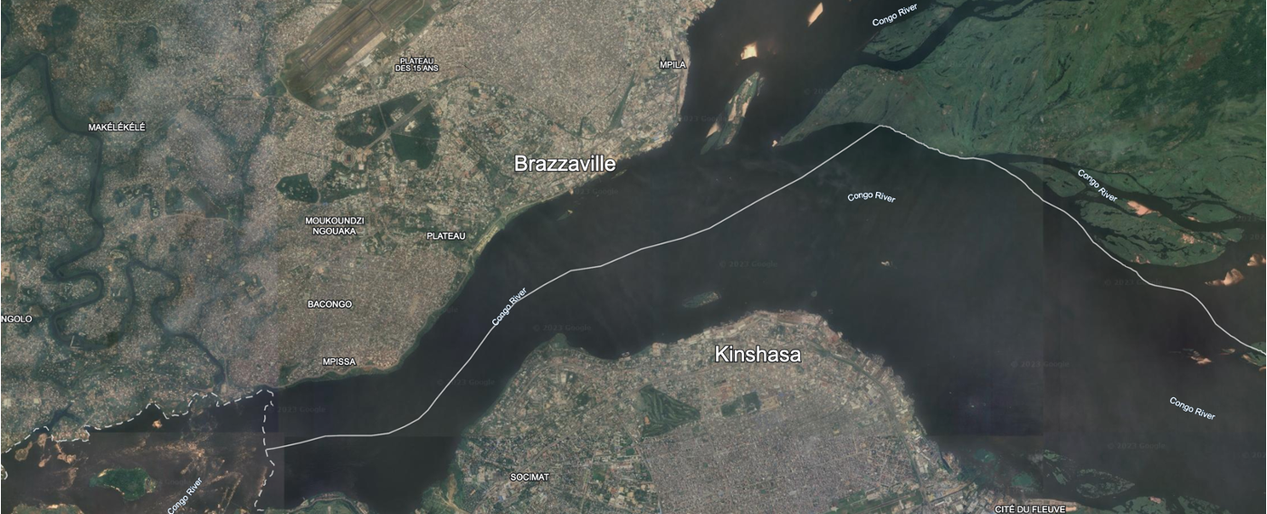
The imprint of human activity on Earth has become unmistakable, offering a unique vantage point for population studies through the lens of space. Access to global high-resolution datasets, such as Landsat(1), has been made possible for the public through platforms like Google Earth Engine (3). These datasets open a window to observe and analyze human settlements, providing invaluable insights into the dynamics of our changing world. The image below is from Google Earth, showing the twin cities of Brazzaville and Kishasa on the banks of the Congo River. One can clearly see the densely package settlements on the banks, along with the unpopulated islands in the river.
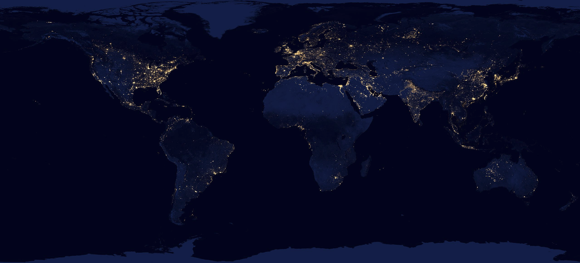
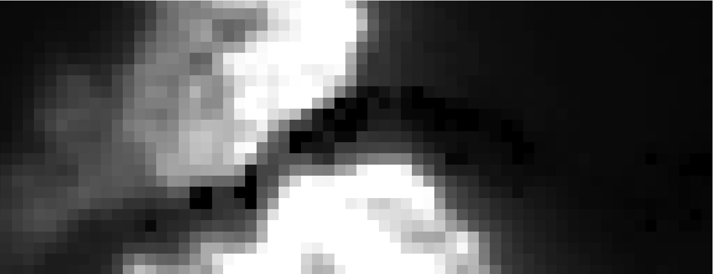
During the night, human presence becomes even more apparent as settlements cast a faint glow into space. This nocturnal illumination is captured by the VIIRS instrument aboard the Suomi National Polar-orbiting Partnership (NPP) satellite. Despite its significance, the relatively weak signals limit the resolution to about 500 meters squared. This limitation poses a challenge to extracting fine-grained information about the distribution and characteristics of human settlements. The image below is of the same area as the one above, but at night. The resolution is significantly lower, with the pixels clearly visible, while the island in the river is completely dark.
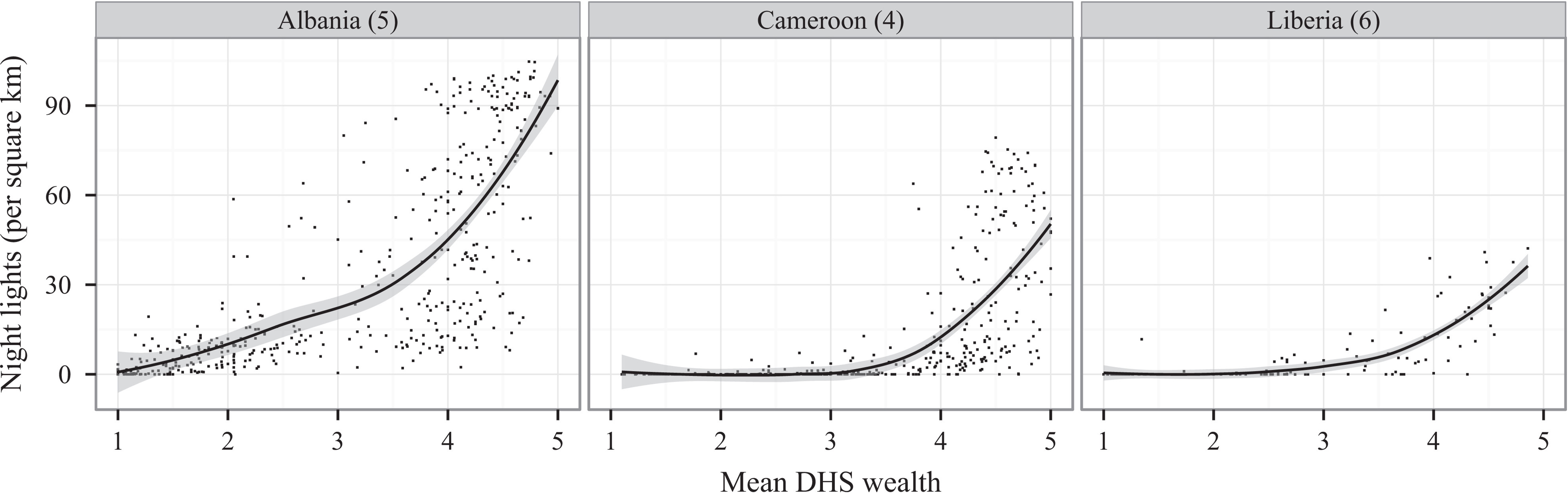
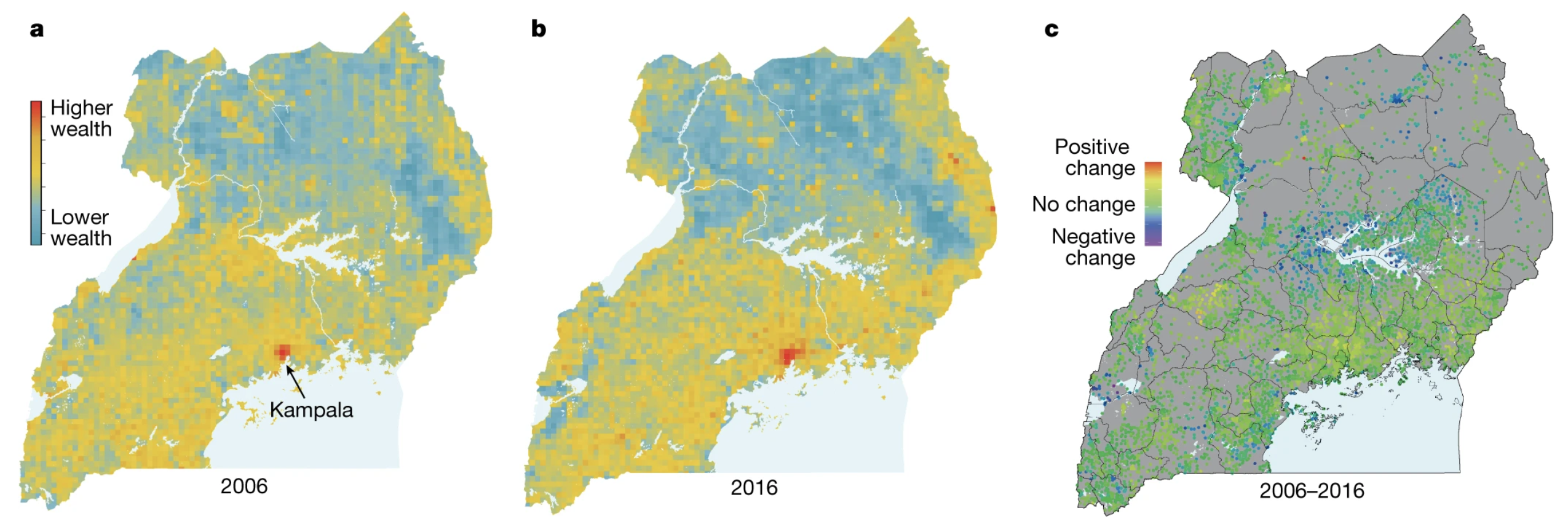
Compelling research underscores the correlation between night lights and mean household wealth, as measured by ground surveys. This correlation establishes night lights as a proxy for gauging livelihoods, making them a valuable tool for socio-economic analyses. This becomes particularly crucial in regions like Sub-Saharan Africa, where traditional population surveys are sparse. The scarcity of on-the-ground data highlights the potential of night lights as a surrogate measure for understanding the economic landscapes of communities. The graph below shows the relationship between night lights and mean household wealth in Sub-Saharan Africa. The data is from the Demographic and Health Surveys (DHS) Program, which conducts household surveys in developing countries. The graph shows a clear correlation between night lights and mean household wealth.
The demand for higher-resolution night lights becomes evident when considering the need for detailed impact assessments. Such assessments can unravel the intricate ways in which individual communities are affected by economic development programs or global events. As technology advances, the quest for sharper and more detailed night light data gains significance, promising to enhance our understanding of human settlements and socio-economic patterns on a global scale. One example of this comes from a paper in Nature just last year that use wealth maps to assess the economic impact of access to electricity. High resolution nightlights would open up even finer grained analysis.
Embarking on this exploration of human settlements and socio-economic patterns, I employ cutting-edge methodologies to surmount the resolution challenges posed by existing night light data. Leveraging the power of machine learning, my approach involves training a model to predict night lights from high-resolution daytime imagery. By undertaking this innovative process, I aim to transcend the limitations of the existing data and generate high-resolution nighttime imagery. This fusion of technological advancements with geospatial analysis not only promises to enrich our understanding of human settlements but also sets the stage for a more nuanced examination of the impact of economic development programs and global events on individual communities. This notebook will serve as a guide for the entire process, from method design to model training and evaluation, and finally, the results and conclusions. The code is available on GitHub.
Methods
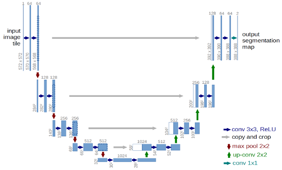
Because I are trying to predict one image from another, I can leverage a Fully Convolutional Network (6) with no dense layers. This allow us to use input imagery of any resolution. The U-Net (7) architecture, named for the shape of the diagram, is the most popular FCN and is well suited to our task. The output layer is modified to perform regression instead of classification so that I get a continuous radiance value instead of segment class. Below is a diagram of U-Net from the original paper -- notice the distintive U shape.
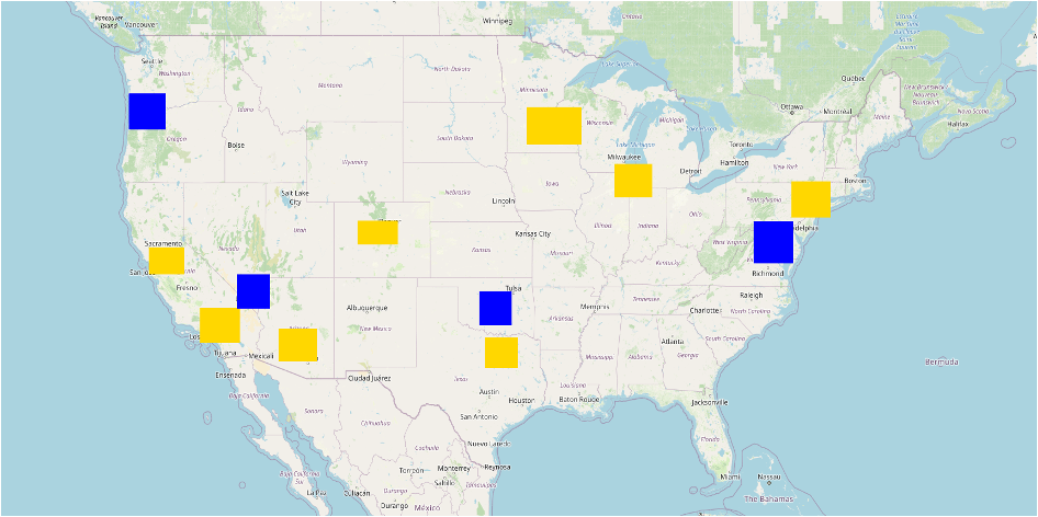
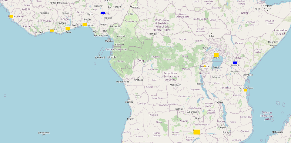
With the model in place, I then need to define our training data. In this project, four different training datasets were tested: both large training regions with 1000 image patch samples from each, as well as small regions with 100 image patch samples from each. Each of these were pulled from the United States and the African continent. For each, there were 8 unique training regions, and 2 evaluation regions. For both areas, the polygons were centered around urban areas, as these have the greatest range of values in nighttime radiance. For consistency, the evaluation areas were also urban areas. Because the target is to predict nightlights in under-surveyed areas, the evaluation sites were Abuja, Nigeria, and Nairobi, Kenya. On the left, I have the large image patches from North America, and on the right from the African. Training patches are in yellow, and evaluation regions are in blue. The aim of having different continents as inputs was to test how transferrable the results are. Do well-lit areas in the US look like well-lit areas in Africa?
| American Cities | African Cities |
|---|---|
 |
 |
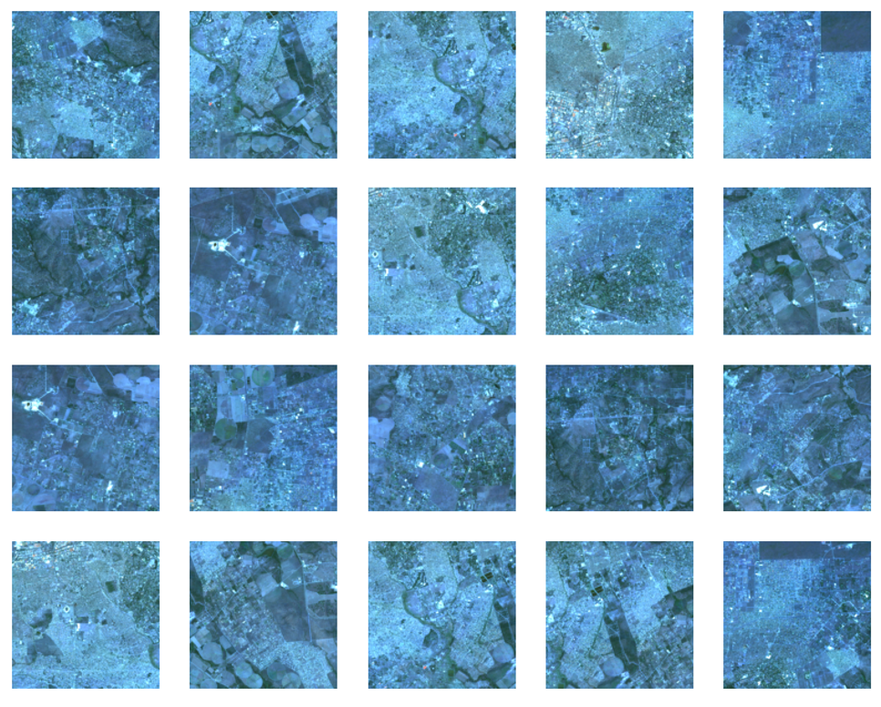
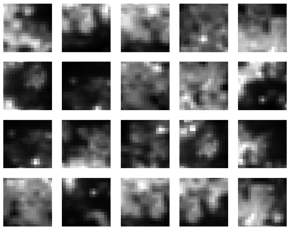
For daytime imagery inputs, I pulled 9 bands from Landsat, 7 optical bands and 2 thermal bands. I created a cloud-masked image composite to create high-quality, cloud free input. For nightlight output, I also create a median composite of the average radiance band from stray-light corrected nightlights.8 The aim is that by pairing each daytime image patch of 256 x 256 with the corresponding nighttime image patch, I can predict nighttime image patches of 128x128 when the original resolution was about 16x16. This is almost 60X improvement in resolution. Below on the left, I have a set of example input images from Landsat in false-color. The level of detail is significant compared with the coarse nightlight image patches on the right.
| Sample Training Inputs | Sample Training Labels |
|---|---|
 |
 |
The other parameters that were experimented with were the number of epochs and the optimizer algorithm. For epochs, values between 1 and 50 were tried for most models. For the optimizer, a single experiment was run with one of the top performing models to see how it would compare. The imagery was compiled in Google Earth Engine via their Python API (9), exported to a Linux computer with a 48GB GPU. The model was built with tensorflow (10), code is available on GitHub (11).
Code for Implementing the Model
Below are the chunks of code to gather the data. To run it yourself, copy and paste the .env.example file to .env and fill in your own file paths and Google Earth Engine credentials. You need an account on Google Cloud Platform with Storage Buckets and access to the Google Earth Engine API to run this, but it can be adapted to export to Google Drive instead before copying it locally.
Configure the Environment
# Read in the .env file
from dotenv import dotenv_values, load_dotenv

# load env variables
config = dotenv_values(".env")
load_dotenv()

# set env variables
GCS_PROJECT = config['GCS_PROJECT']
BUCKET = config['BUCKET']
HOME_PATH = config['HOME_PATH']
LOCAL_PATH = config['LOCAL_PATH']
DATA_PATH = config['DATA_PATH']
FOLDER = config['FOLDER']
GCLOUD_PATH = config['GCLOUD_PATH']
CUDA_VISIBLE_DEVICES = config['CUDA_VISIBLE_DEVICES']

print(config)
OrderedDict([('GCS_PROJECT', 'master-thesis-ilg'), ('BUCKET', 'csci5922-proj'), ('HOME_PATH', '/home/isly9493/'), ('LOCAL_PATH', '/local/isly9493/'), ('DATA_PATH', 'csci5922/proj/data/'), ('FOLDER', 'viirs-africa-many/'), ('GCLOUD_PATH', '/home/isly9493/google-cloud-sdk/bin/'), ('CUDA_VISIBLE_DEVICES', '1')])
Import Key Libraries and Authenticate to Google Earth Engine
We use Earth Engine to fetch, process, and display our imagery. We use tensorflow to build and train our model. Finally, we use folium to create interactive maps to display our results.
# Import, authenticate and initialize the Earth Engine library.
import ee
ee.Authenticate()
ee.Initialize()

# Tensorflow setup.
import tensorflow as tf
print(tf.__version__)

# Folium setup.
import folium
print(folium.__version__)

# supress warnings
import warnings
warnings.filterwarnings('ignore')
2.15.0
0.15.1
Set other Global Variables
# variables for image names
TRAINING_BASE = 'training_patches'
EVAL_BASE = 'eval_patches'

# Specify inputs (Landsat bands) to the model and the response variable.
opticalBands = ['B1', 'B2', 'B3', 'B4', 'B5', 'B6', 'B7']
thermalBands = ['B10', 'B11']
BANDS = opticalBands + thermalBands
RESPONSE = 'avg_rad' #####
FEATURES = BANDS + [RESPONSE]

# Specify the size and shape of patches expected by the model.
KERNEL_SIZE = 256
KERNEL_SHAPE = [KERNEL_SIZE, KERNEL_SIZE]
COLUMNS = [
  tf.io.FixedLenFeature(shape=KERNEL_SHAPE, dtype=tf.float32) for k in FEATURES
]
FEATURES_DICT = dict(zip(FEATURES, COLUMNS))

# Sizes of the training and evaluation datasets.
TRAIN_SIZE = 4800
EVAL_SIZE = 200

# Specify model training parameters.
BATCH_SIZE = 48
EPOCHS = 1
BUFFER_SIZE = 2000
OPTIMIZER = 'SGD'
LOSS = 'MeanSquaredError'
METRICS = ['RootMeanSquaredError']
Data Preparation
Gather and setup the imagery to use for inputs (predictors). This is a three-year, cloud-free, Landsat 8 composite. Display it in the notebook for a sanity check.
# Use Landsat 8 surface reflectance data.
l8sr = ee.ImageCollection('LANDSAT/LC08/C01/T1_SR')
# Cloud masking function.
def maskL8sr(image):
cloudShadowBitMask = ee.Number(2).pow(3).int()
cloudsBitMask = ee.Number(2).pow(5).int()
qa = image.select('pixel_qa')
mask1 = qa.bitwiseAnd(cloudShadowBitMask).eq(0).And(
qa.bitwiseAnd(cloudsBitMask).eq(0))
mask2 = image.mask().reduce('min')
mask3 = image.select(opticalBands).gt(0).And(
image.select(opticalBands).lt(10000)).reduce('min')
mask = mask1.And(mask2).And(mask3)
return image.select(opticalBands).divide(10000).addBands(
image.select(thermalBands).divide(10).clamp(273.15, 373.15)
.subtract(273.15).divide(100)).updateMask(mask)
# The image input data is a cloud-masked median composite.
image = l8sr.filterDate('2020-01-01', '2022-12-31').map(maskL8sr).median()
# printn out the bands
print(image.bandNames().getInfo())
# Use folium to visualize the imagery.
mapid = image.getMapId({'bands': ['B4', 'B3', 'B2'], 'min': 0, 'max': 0.3})
map = folium.Map(location=[-1, 37], zoom_start=6)
folium.TileLayer(
tiles=mapid['tile_fetcher'].url_format,
attr='Map Data © <a href="https://earthengine.google.com/">Google Earth Engine</a>',
overlay=True,
name='median composite',
).add_to(map)
mapid = image.getMapId({'bands': ['B10'], 'min': 0, 'max': 0.5})
folium.TileLayer(
tiles=mapid['tile_fetcher'].url_format,
attr='Map Data © <a href="https://earthengine.google.com/">Google Earth Engine</a>',
overlay=True,
name='thermal',
).add_to(map)
map.add_child(folium.LayerControl())
map
['B1', 'B2', 'B3', 'B4', 'B5', 'B6', 'B7', 'B10', 'B11']
Prepare the response (what we want to predict). This is nighttime brightness (in nanoWatts/sr/cm^2) from the VIIRS dataset. Display to check.
viirs = ee.ImageCollection('NOAA/VIIRS/DNB/MONTHLY_V1/VCMSLCFG').select('avg_rad').filterDate('2020-01-01', '2022-12-31').median()
viirs = viirs.divide(60).float() # normalize to 0-1 range
mapid = viirs.getMapId({'min': 0, 'max': 0.02})
map = folium.Map(location=[-1, 37], zoom_start=6)
folium.TileLayer(
tiles=mapid['tile_fetcher'].url_format,
attr='Map Data © <a href="https://earthengine.google.com/">Google Earth Engine</a>',
overlay=True,
name='viirs dnb',
).add_to(map)
map.add_child(folium.LayerControl())
map
Stack the 2D images (Landsat composite and VIIRS DNB image) to create a single image from which samples can be taken. Convert the image into an array image in which each pixel stores 256x256 patches of pixels for each band. This is a key step that bears emphasis: to export training patches, convert a multi-band image to an array image using neighborhoodToArray(), then sample the image at points.
featureStack = ee.Image.cat([
  image.select(BANDS),
  viirs.select(RESPONSE)
]).float()

list = ee.List.repeat(1, KERNEL_SIZE)
lists = ee.List.repeat(list, KERNEL_SIZE)
kernel = ee.Kernel.fixed(KERNEL_SIZE, KERNEL_SIZE, lists)

arrays = featureStack.neighborhoodToArray(kernel)
Define Training and Evaluation Areas
Use some pre-made geometries to sample the stack in strategic locations. Specifically, these are hand-made polygons in which to take the 256x256 samples. Display the sampling polygons on a map, red for training polygons, blue for evaluation. You'll need to create these polygons ahead of time yourself and save them as a feature collection. This is easiest to do in Google Earth Engine's code editor, but can also be done via the API.
trainingPolys = ee.FeatureCollection('projects/'+GCS_PROJECT+'/assets/trainingPolysAfricaBig')
evalPolys = ee.FeatureCollection('projects/'+GCS_PROJECT+'/assets/evalPolysAfrica')
polyImage = ee.Image(0).byte().paint(trainingPolys, 1).paint(evalPolys, 2)
polyImage = polyImage.updateMask(polyImage)
mapid = polyImage.getMapId({'min': 1, 'max': 2, 'palette': ['gold', 'blue']})
map = folium.Map(location=[0, 12], zoom_start=5)
folium.TileLayer(
tiles=mapid['tile_fetcher'].url_format,
attr='Map Data © <a href="https://earthengine.google.com/">Google Earth Engine</a>',
overlay=True,
name='training polygons',
).add_to(map)
map.add_child(folium.LayerControl())
map
Sampling
The mapped data look reasonable so take a sample from each polygon and merge the results into a single export. The key step is sampling the array image at points, to get all the pixels in a 256x256 neighborhood at each point. It's worth noting that to build the training and testing data for the FCNN, you export a single TFRecord file that contains patches of pixel values in each record. You do not need to export each training/testing patch to a different image. Since each record potentially contains a lot of data (especially with big patches or many input bands), some manual sharding of the computation is necessary to avoid the computed value too large error. Specifically, the following code takes multiple (smaller) samples within each geometry, merging the results to get a single export.
# Convert the feature collections to lists for iteration.
trainingPolysList = trainingPolys.toList(trainingPolys.size())
evalPolysList = evalPolys.toList(evalPolys.size())

# These numbers determined experimentally.
n = 20 # Number of shards in each polygon.
N = 200 # Total sample size in each polygon.
Export Training & Evaluation Data from Earth Engine to Google Cloud Storage
This can be modified to export to local storage, just adjust the file paths.
# Export all the training data (in many pieces), with one task
# per geometry.
for g in range(trainingPolys.size().getInfo()):
  geomSample = ee.FeatureCollection([])
  for i in range(n):
    sample = arrays.sample(
      region = ee.Feature(trainingPolysList.get(g)).geometry(),
      scale = 30,
      numPixels = N / n, # Size of the shard.
      seed = i,
      tileScale = 8
    )
    geomSample = geomSample.merge(sample)

  desc = TRAINING_BASE + '_g' + str(g)
  print(g, FOLDER, BUCKET, desc)

  task = ee.batch.Export.table.toCloudStorage(
    collection = geomSample,
    description = desc,
    bucket = BUCKET,
    fileNamePrefix = FOLDER + desc,
    fileFormat = 'TFRecord',
    selectors = BANDS + [RESPONSE]
  )
  task.start()
print('Training imagery tasks submitted. Check on the Tasks in GEE for their status (https://code.earthengine.google.com/tasks).')
# Export all the evaluation data.
for g in range(evalPolys.size().getInfo()):
  geomSample = ee.FeatureCollection([])
  for i in range(n):
    sample = arrays.sample(
      region = ee.Feature(evalPolysList.get(g)).geometry(),
      scale = 30,
      numPixels = N / n,
      seed = i,
      tileScale = 8
    )
    geomSample = geomSample.merge(sample)

  desc = EVAL_BASE + '_g' + str(g)
  print(g, FOLDER, BUCKET, desc)

  task = ee.batch.Export.table.toCloudStorage(
    collection = geomSample,
    description = desc,
    bucket = BUCKET,
    fileNamePrefix = FOLDER + desc,
    fileFormat = 'TFRecord',
    selectors = BANDS + [RESPONSE]
  )
  task.start()
print('Eval imagery tasks submitted. Check on the Tasks in GEE for their status (https://code.earthengine.google.com/tasks).')
Copy Files from Google Cloud Storage to Local Storage
This moves the files to the local machine for training. Note that you need the Google Cloud SDK installed and authenticated to run this.
# Copy from your bucket to local path (note -r is for recursive call)
!{GCLOUD_PATH}gsutil -m cp -r 'gs://'{BUCKET}'/'{FOLDER}{TRAINING_BASE}'*' {LOCAL_PATH}{DATA_PATH}{FOLDER}
!{GCLOUD_PATH}gsutil -m cp -r 'gs://'{BUCKET}'/'{FOLDER}{EVAL_BASE}'*' {LOCAL_PATH}{DATA_PATH}{FOLDER}
Configure GPU Usage
Use this to ensure you are using the GPUs that you intend for training. This assumes you have CUDA and cuDNN installed.
# see what devices are available
print("Num GPUs Available: ", len(tf.config.list_physical_devices('GPU')))
print("GPUs Available: ", tf.config.list_physical_devices('GPU'))
!nvidia-smi
Num GPUs Available:  1
GPUs Available:  [PhysicalDevice(name='/physical_device:GPU:0', device_type='GPU')]
2023-12-12 16:01:15.741987: I external/local_xla/xla/stream_executor/cuda/cuda_executor.cc:901] successful NUMA node read from SysFS had negative value (-1), but there must be at least one NUMA node, so returning NUMA node zero. See more at https://github.com/torvalds/linux/blob/v6.0/Documentation/ABI/testing/sysfs-bus-pci#L344-L355
2023-12-12 16:01:15.773299: I external/local_xla/xla/stream_executor/cuda/cuda_executor.cc:901] successful NUMA node read from SysFS had negative value (-1), but there must be at least one NUMA node, so returning NUMA node zero. See more at https://github.com/torvalds/linux/blob/v6.0/Documentation/ABI/testing/sysfs-bus-pci#L344-L355
2023-12-12 16:01:15.773568: I external/local_xla/xla/stream_executor/cuda/cuda_executor.cc:901] successful NUMA node read from SysFS had negative value (-1), but there must be at least one NUMA node, so returning NUMA node zero. See more at https://github.com/torvalds/linux/blob/v6.0/Documentation/ABI/testing/sysfs-bus-pci#L344-L355
Load Training and Evaluation Data in Memory for Training.
Load the data exported from Earth Engine into a tf.data.Dataset. The following are helper functions for that.
def parse_tfrecord(example_proto):
  return tf.io.parse_single_example(example_proto, FEATURES_DICT)


def to_tuple(inputs):
  inputsList = [inputs.get(key) for key in FEATURES]
  stacked = tf.stack(inputsList, axis=0)
  # Convert from CHW to HWC
  stacked = tf.transpose(stacked, [1, 2, 0])
  return stacked[:,:,:len(BANDS)], stacked[:,:,len(BANDS):]


def get_dataset(path, prefix, n_files):
  glob = []
  for i in range(0, n_files):
    glob = path + prefix + '_g' + str(i) + '.tfrecord.gz'
  dataset = tf.data.TFRecordDataset(glob, compression_type='GZIP')
  dataset = dataset.map(parse_tfrecord, num_parallel_calls=5)
  dataset = dataset.map(to_tuple, num_parallel_calls=5)
  return dataset
Use the helpers to read in the training dataset. Optionally print the first record to check. Careful, this will make tensorflow reserve as much GPU memory as is available to it.
training = get_dataset(LOCAL_PATH + DATA_PATH + FOLDER, TRAINING_BASE, 24)
training = training.shuffle(BUFFER_SIZE).batch(BATCH_SIZE).repeat()
# print(iter(training.take(1)).next())
Evaluation data
Now do the same thing to get an evaluation dataset. Note that unlike the training dataset, the evaluation dataset has a batch size of 1, is not repeated and is not shuffled.
evaluation = get_dataset(LOCAL_PATH + DATA_PATH + FOLDER, EVAL_BASE, 2)
evaluation = evaluation.batch(1).repeat()
# print(iter(evaluation.take(1)).next()[0][0,:,:,1:3])
# visualize of the of the training / evaluation image patch pairs
import numpy as np
import matplotlib.pyplot as plt

def display_batch_of_images(databatch):
    imgs, labels = databatch
    # landsat in false color
    plt.figure(figsize=(10,10))
    label = labels.numpy().astype(np.float32)
    for i in range(25):
        plt.subplot(5,5,i+1)
        plt.imshow(imgs[i,:,:,0:3]*8) # select landsat bands here
        plt.axis('off')
    plt.show()
    # show viirs in grayscale
    plt.figure(figsize=(10,10))
    for i in range(25):
        plt.subplot(5,5,i+1)
        plt.imshow(labels[i,:,:,0], cmap='gray')
        plt.axis('off')
    plt.show()

display_batch_of_images(iter(training.take(1)).next())
Clipping input data to the valid range for imshow with RGB data ([0..1] for floats or [0..255] for integers).
Clipping input data to the valid range for imshow with RGB data ([0..1] for floats or [0..255] for integers).
Clipping input data to the valid range for imshow with RGB data ([0..1] for floats or [0..255] for integers).
Clipping input data to the valid range for imshow with RGB data ([0..1] for floats or [0..255] for integers).
Clipping input data to the valid range for imshow with RGB data ([0..1] for floats or [0..255] for integers).
Clipping input data to the valid range for imshow with RGB data ([0..1] for floats or [0..255] for integers).
Clipping input data to the valid range for imshow with RGB data ([0..1] for floats or [0..255] for integers).
Clipping input data to the valid range for imshow with RGB data ([0..1] for floats or [0..255] for integers).
Clipping input data to the valid range for imshow with RGB data ([0..1] for floats or [0..255] for integers).
Clipping input data to the valid range for imshow with RGB data ([0..1] for floats or [0..255] for integers).
Clipping input data to the valid range for imshow with RGB data ([0..1] for floats or [0..255] for integers).
Clipping input data to the valid range for imshow with RGB data ([0..1] for floats or [0..255] for integers).
Clipping input data to the valid range for imshow with RGB data ([0..1] for floats or [0..255] for integers).
Clipping input data to the valid range for imshow with RGB data ([0..1] for floats or [0..255] for integers).
Clipping input data to the valid range for imshow with RGB data ([0..1] for floats or [0..255] for integers).
Clipping input data to the valid range for imshow with RGB data ([0..1] for floats or [0..255] for integers).
Clipping input data to the valid range for imshow with RGB data ([0..1] for floats or [0..255] for integers).
Clipping input data to the valid range for imshow with RGB data ([0..1] for floats or [0..255] for integers).


Data Analysis & Deep Learning Model
Here we use the Keras implementation of the U-Net model. The U-Net model takes 256x256 pixel patches as input and outputs per-pixel class probability, label or a continuous output. We can implement the model essentially unmodified, but will use mean squared error loss on the sigmoidal output since we are treating this as a regression problem, rather than a classification problem.
from tensorflow import keras
from keras import layers
from keras import losses
from keras import models
from keras import metrics
from keras import optimizers

def conv_block(input_tensor, num_filters):
	encoder = layers.Conv2D(num_filters, (3, 3), padding='same')(input_tensor)
	encoder = layers.BatchNormalization()(encoder)
	encoder = layers.Activation('relu')(encoder)
	encoder = layers.Conv2D(num_filters, (3, 3), padding='same')(encoder)
	encoder = layers.BatchNormalization()(encoder)
	encoder = layers.Activation('relu')(encoder)
	return encoder

def encoder_block(input_tensor, num_filters):
	encoder = conv_block(input_tensor, num_filters)
	encoder_pool = layers.MaxPooling2D((2, 2), strides=(2, 2))(encoder)
	return encoder_pool, encoder


def decoder_block(input_tensor, concat_tensor, num_filters):
	decoder = layers.Conv2DTranspose(num_filters, (2, 2), strides=(2, 2), padding='same')(input_tensor)
	decoder = layers.concatenate([concat_tensor, decoder], axis=-1)
	decoder = layers.BatchNormalization()(decoder)
	decoder = layers.Activation('relu')(decoder)
	decoder = layers.Conv2D(num_filters, (3, 3), padding='same')(decoder)
	decoder = layers.BatchNormalization()(decoder)
	decoder = layers.Activation('relu')(decoder)
	decoder = layers.Conv2D(num_filters, (3, 3), padding='same')(decoder)
	decoder = layers.BatchNormalization()(decoder)
	decoder = layers.Activation('relu')(decoder)
	return decoder

def get_model():
	inputs = layers.Input(shape=[None, None, len(BANDS)]) # 256
	encoder0_pool, encoder0 = encoder_block(inputs, 32) # 128
	encoder1_pool, encoder1 = encoder_block(encoder0_pool, 64) # 64
	encoder2_pool, encoder2 = encoder_block(encoder1_pool, 128) # 32
	encoder3_pool, encoder3 = encoder_block(encoder2_pool, 256) # 16
	encoder4_pool, encoder4 = encoder_block(encoder3_pool, 512) # 8
	center = conv_block(encoder4_pool, 1024) # center
	decoder4 = decoder_block(center, encoder4, 512) # 16
	decoder3 = decoder_block(decoder4, encoder3, 256) # 32
	decoder2 = decoder_block(decoder3, encoder2, 128) # 64
	decoder1 = decoder_block(decoder2, encoder1, 64) # 128
	decoder0 = decoder_block(decoder1, encoder0, 32) # 256

	# to change your output activation function, change this part
	outputs = layers.Conv2D(1, (1, 1), activation='sigmoid')(decoder0)

	model = models.Model(inputs=[inputs], outputs=[outputs])

	# set optimizer with custom learning rate
	OPTIMIZER = 'SGD'
	optimizer = optimizers.get(OPTIMIZER)

	# to adjust the learning rate:
	# optimizer.learning_rate = 0.1

	# compile the model
	model.compile(
		optimizer=optimizer,
		loss=losses.get(LOSS),
		metrics=[metrics.get(metric) for metric in METRICS])

	return model
Training the model
You train a Keras model by calling .fit() on it. Here we're going to train for 10 epochs, which is suitable for demonstration purposes. For production use, you probably want to optimize this parameter, for example through hyperparamter tuning.
# print the current time to log how long it takes to train
from datetime import datetime
print(datetime.now())

# get the model fresh and train it
m = get_model()
history = m.fit(
    x=training,
    epochs=EPOCHS,
    steps_per_epoch=int(TRAIN_SIZE / BATCH_SIZE),
    validation_data=evaluation,
    validation_steps=EVAL_SIZE
)

# print the end time to log how long it takes to train
print(datetime.now())
2023-12-12 16:18:50.358788
100/100 [==============================] - 42s 361ms/step - loss: 0.2118 - root_mean_squared_error: 0.4602 - val_loss: 0.1753 - val_root_mean_squared_error: 0.4187
2023-12-12 16:19:33.359108
# set some parameters for saving the model
MODEL_NAME = 'viirs_africa_many_e1.keras'
HISTORY_NAME = 'viirs_africa_many_e1_history.pickle'
ASSET_SUFFIX = 'viirs_africa_many_e1'
# save the model to a local file
m.save(LOCAL_PATH + DATA_PATH + FOLDER + MODEL_NAME)

# # save the history variable to a local file with pickle
import pickle
with open(LOCAL_PATH + DATA_PATH + FOLDER + HISTORY_NAME, 'wb') as f:
  pickle.dump(history, f)

# import a saved model if needed
# m = tf.keras.models.load_model(LOCAL_PATH + DATA_PATH + FOLDER + MODEL_NAME)
# import pickle
# with open(HISTORY_NAME, 'rb') as f:
# with open(LOCAL_PATH + DATA_PATH + FOLDER + HISTORY_NAME, 'rb') as f:
#   history = pickle.load(f)
Evaluation
Let's look at how the model performed in terms of loss while it trained, and then evaluate it on the training and evaluation datasets.
# plot the training and validation loss
import matplotlib.pyplot as plt

plt.plot(history.history['root_mean_squared_error'])
plt.plot(history.history['val_root_mean_squared_error'])
plt.title('Model RMSE for ' + ASSET_SUFFIX + ' for ' + str(EPOCHS) + ' epochs')
plt.ylabel('RMSE')
plt.xlabel('Epoch')
plt.legend(['Training RMSE', 'Validation RMSE'], loc='upper left')
plt.show()

## evaluate the model on the evaluation dataset to get the loss and RMSE
val_loss, val_rmse = m.evaluate(evaluation, steps=EVAL_SIZE)
print('Model validation loss: {:0.4f}. RMSE: {:0.4f}'.format(val_loss, val_rmse))
200/200 [==============================] - 1s 7ms/step - loss: 0.1753 - root_mean_squared_error: 0.4187
Model validation loss: 0.1753. RMSE: 0.4187
## evaluate the model on the evaluation dataset to get the loss and RMSE
train_loss, train_rmse = m.evaluate(training, steps=10)
print('Model train loss: {:0.4f}. RMSE: {:0.4f}'.format(train_loss, train_rmse))
10/10 [==============================] - 3s 212ms/step - loss: 0.2333 - root_mean_squared_error: 0.4830
Model train loss: 0.2333. RMSE: 0.4830
Prediction
Now we're going to do a qualitative assessment of the model by running it on an input image patch, specifically Brazzaville / Kinshasa. The prediction pipeline is:
- Export imagery on which to do predictions from Earth Engine in TFRecord format to a Cloud Storage bucket.
- Use the trained model to make the predictions.
- Write the predictions to a TFRecord file in a Cloud Storage.
- Upload the predictions TFRecord file to Earth Engine.
Specify Region and Outputs for Prediction
ee_user_folder = 'projects/'+GCS_PROJECT+'/assets'

pred_image_base = 'FCNN_demo_kinshasa_384_'
# Half this will extend on the sides of each patch.
pred_kernel_buffer = [128, 128]
# Kinshasa/Brazzaville
pred_region = ee.Geometry.Polygon(
  [[[15.02, -4.04],
    [15.02, -4.54],
    [15.52, -4.54],
    [15.52, -4.04]]],
  None,
  False
)
Export Sample Imagery for Prediction
This only needs to be run once. It exports the sample imagery to a TFRecord file in a Cloud Storage bucket.
def doExport(out_image_base, kernel_buffer, region):
  task = ee.batch.Export.image.toCloudStorage(
    image = image.select(BANDS),
    description = out_image_base,
    bucket = BUCKET,
    fileNamePrefix = FOLDER + out_image_base,
    region = region.getInfo()['coordinates'],
    scale = 30,
    fileFormat = 'TFRecord',
    maxPixels = 1e10,
    formatOptions = {
      'patchDimensions': KERNEL_SHAPE,
      'kernelSize': kernel_buffer,
      'compressed': True,
      'maxFileSize': 104857600
    }
  )
  task.start()
  print('Prediction image export task submitted. Check on the task in GEE for its status (https://code.earthengine.google.com/tasks).')
# Run the export.
doExport(pred_image_base, pred_kernel_buffer, pred_region)
Prediction image export task submitted. Check on the task in GEE for its status (https://code.earthengine.google.com/tasks).
# copy the prediction file from cloud storage to local
!{GCLOUD_PATH}gsutil -m cp -r 'gs://'{BUCKET}'/'{FOLDER}{pred_image_base}'*' {LOCAL_PATH}{DATA_PATH}{FOLDER}
Define Code for Running Model on Prediction Data
Expects the prediction data to exist locally.
def doPrediction(out_image_base, kernel_buffer):
  print('Looking for TFRecord files...')

  # # Get a list of all the files in the output bucket.
  filesList = !ls {LOCAL_PATH}{DATA_PATH}{FOLDER}

  # Get only the files generated by the image export.
  exportFilesList = [s for s in filesList if out_image_base in s]

  # Get the list of image files and the JSON mixer file.
  imageFilesList = []
  jsonFile = None
  for f in exportFilesList:
    if f.endswith('.tfrecord.gz'):
      imageFilesList.append(f)
    elif f.endswith('.json'):
      jsonFile = f
  imageFilesList.sort()

  from pprint import pprint
  pprint(imageFilesList)
  print(jsonFile)

  import json
  jsonText = !cat {LOCAL_PATH}{DATA_PATH}{FOLDER}{jsonFile}
  print(jsonText)
  mixer = json.loads(jsonText.nlstr)
  pprint(mixer)
  patches = mixer['totalPatches']

  buffered_shape = [
      KERNEL_SHAPE[0] + kernel_buffer[0],
      KERNEL_SHAPE[1] + kernel_buffer[1]]

  imageColumns = [
    tf.io.FixedLenFeature(shape=buffered_shape, dtype=tf.float32)
      for k in BANDS
  ]

  imageFeaturesDict = dict(zip(BANDS, imageColumns))

  def parse_image(example_proto):
    return tf.io.parse_single_example(example_proto, imageFeaturesDict)

  def toTupleImage(inputs):
    inputsList = [inputs.get(key) for key in BANDS]
    stacked = tf.stack(inputsList, axis=0)
    stacked = tf.transpose(stacked, [1, 2, 0])
    return stacked

  # append absolute path to imageFilesList
  imageFilesList = [LOCAL_PATH + DATA_PATH + FOLDER + f for f in imageFilesList]
  print(imageFilesList)

  # Create a dataset from the TFRecord file(s) in Cloud Storage.
  imageDataset = tf.data.TFRecordDataset(imageFilesList, compression_type='GZIP')
  imageDataset = imageDataset.map(parse_image, num_parallel_calls=5)
  imageDataset = imageDataset.map(toTupleImage).batch(1)

  # Perform inference.
  print('Running predictions...')
  predictions = m.predict(imageDataset, steps=patches, verbose=1)
  # print(predictions[0])
  return predictions
def writePredictions(predictions, out_image_base, kernel_buffer):
  print('Writing predictions...')
  out_image_file = 'gs://' + BUCKET + '/' + FOLDER + out_image_base + '.TFRecord'

  # Get set up for prediction.
  x_buffer = int(kernel_buffer[0] / 2)
  y_buffer = int(kernel_buffer[1] / 2)


  writer = tf.io.TFRecordWriter(out_image_file)
  patches = 0
  for predictionPatch in predictions:
    # print('Writing patch ' + str(patches) + '...')
    predictionPatch = predictionPatch[
        x_buffer:x_buffer+KERNEL_SIZE, y_buffer:y_buffer+KERNEL_SIZE]

    # Create an example.
    example = tf.train.Example(
      features=tf.train.Features(
        feature={
          'impervious': tf.train.Feature(
            float_list=tf.train.FloatList(
              value=predictionPatch.flatten()
            )
          )
        }
      )
    )
    # Write the example.
    writer.write(example.SerializeToString())
    patches += 1

  print('Done writing predictions.')
  writer.close()
def uploadPredictionsToEE(out_image_base, ee_user_folder):
  # Start the upload.
  print('Uploading to Google Earth Egnine...')

  # define file paths
  out_image_file = 'gs://' + BUCKET + '/' + FOLDER + out_image_base + '.TFRecord'
  out_image_asset = ee_user_folder + '/' + out_image_base + ASSET_SUFFIX
  jsonFile = 'gs://' + BUCKET + '/' + FOLDER + out_image_base + 'mixer.json'

  print('out_image_asset: ', out_image_asset)
  print('out_image_file: ', out_image_file)
  print('jsonFile: ', jsonFile)

  # upload file to google earth engine from gcs
  !earthengine upload image --asset_id={out_image_asset} {out_image_file} {jsonFile}

  print('Prediction image upload task submitted. Check on the task in GEE for its status (https://code.earthengine.google.com/tasks).')
Run Predictions
# Run the prediction.
predictions = doPrediction(pred_image_base, pred_kernel_buffer)
# Write the predictions.
writePredictions(predictions, pred_image_base, pred_kernel_buffer)
# upload to earth engine
uploadPredictionsToEE(pred_image_base, ee_user_folder)
Display the Prediction
One the data has been exported, the model has made predictions and the predictions have been written to a file, and the image imported to Earth Engine, it's possible to display the resultant Earth Engine asset.
map = folium.Map(location=[-4.29, 15.27], zoom_start=11)
# add landsat layer clipped to prediction region
landsat = image
landsat = landsat.clip(pred_region)
mapid = landsat.getMapId({'bands': ['B4', 'B3', 'B2'], 'min': 0, 'max': 0.3})
folium.TileLayer(
tiles=mapid['tile_fetcher'].url_format,
attr='Map Data © <a href="https://earthengine.google.com/">Google Earth Engine</a>',
overlay=True,
name='landsat',
).add_to(map)
# actual viirs
viirs = ee.ImageCollection('NOAA/VIIRS/DNB/MONTHLY_V1/VCMSLCFG').select('avg_rad').filterDate('2021-01-01', '2022-12-31').median().divide(30).float()
viirs = viirs.clip(pred_region)
# actual_image = viirs
mapid = viirs.getMapId({'min': 0, 'max': 1}) # normally max 1.0
folium.TileLayer(
tiles=mapid['tile_fetcher'].url_format,
attr='Map Data © <a href="https://earthengine.google.com/">Google Earth Engine</a>',
overlay=True,
name='viirs dnb',
).add_to(map)
# prediction
out_image = ee.Image(ee_user_folder + '/' + pred_image_base + ASSET_SUFFIX)
mapid = out_image.getMapId({'min': 0, 'max': 1})
folium.TileLayer(
tiles=mapid['tile_fetcher'].url_format,
attr='Map Data © <a href="https://earthengine.google.com/">Google Earth Engine</a>',
overlay=True,
name='predicted nightlights',
).add_to(map)
# difference
diff = out_image.subtract(viirs)
mapid = diff.getMapId({'min': -0.5, 'max': 0.5, 'palette': ['FF0000', '000000', '00FF00']})
folium.TileLayer(
tiles=mapid['tile_fetcher'].url_format,
attr='Map Data © <a href="https://earthengine.google.com/">Google Earth Engine</a>',
overlay=True,
name='difference',
).add_to(map)
# visualize the map
map.add_child(folium.LayerControl())
map
Results
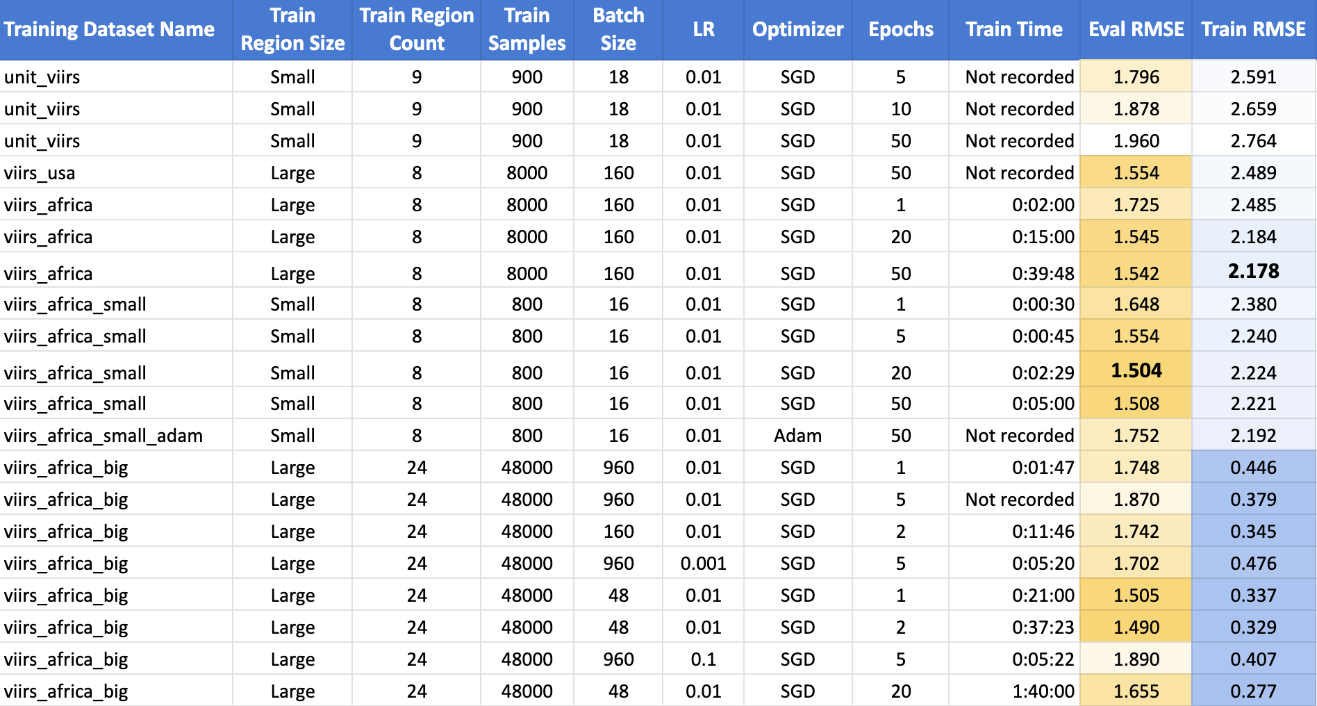
The top performing model was the one trained on the small polygons around African cities for 20 epochs using Stochastic Gradient Descent, achieving an RMSE of 1.504. Surprisingly, increasing the samples in the training dataset by 10X did not improve on the results. Another surprise is that the train RMSE was consistently lower than the validation RMSE. This is highly atypical, and suggests that there is an issue with the training strategy. The full table of results is below.
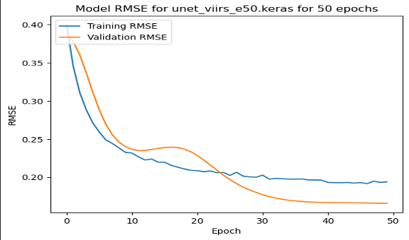
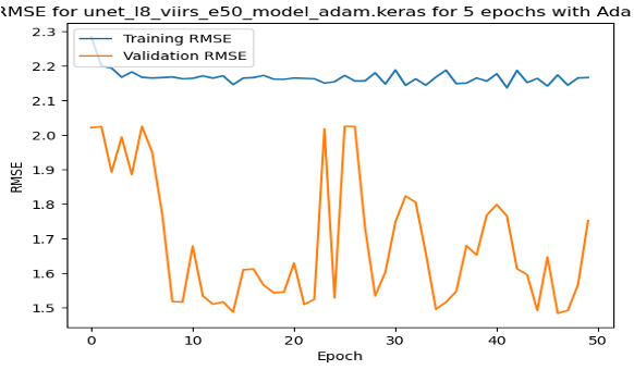
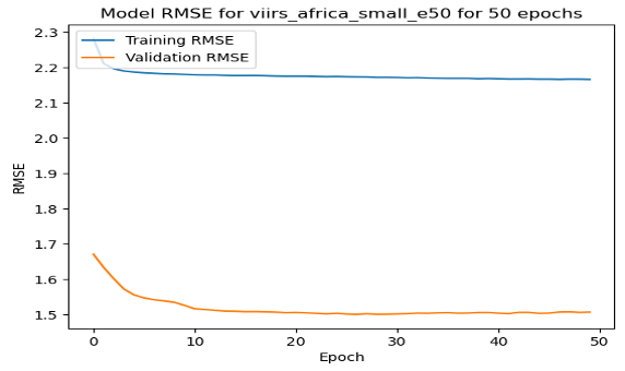
On these RMSE by epoch graphs, we have a few interesting results. (1) shows the model training and validating in the USA, the only one where validation error followed a more regular trend. (2) shows the training with the Adam Optimizer, showing quite unstable training. (3) shows the stable training of one of the top performing models. However, it reaches quite close to the minimum in just about 15 epochs, and does not improve from there.
| Loss by Epoch for Small USA 50 Epochs | Loss by Epoch for Small African Cities with Adam Optimizer | Loss by Epoch for Small African Cities with SGD Optimizer |
|---|---|---|
 |
 |
 |
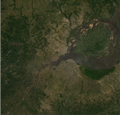
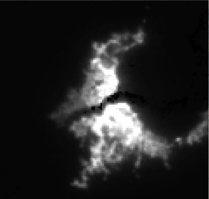
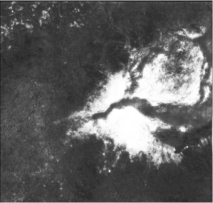
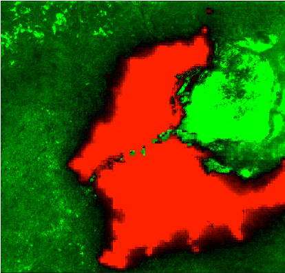
Finally, for each model, I ran a prediction pipeline for an untrained area, the twin cities of Kinshasa and Brazzaville between the Congo and the Democratic Republic of Congo for a qualitiative analysis. (1) shows the true color Landsat composite, (2) shows the VIIRS nightlights, (3) shows the predicted nightlights, and (4) shows the difference between (2) and (3). On this prediction, the model is picking up the features of urbanization in the cities, but it falsely classifies the island in the river delta as well lit while it is not populated.
| Input Landsat Image | VIIRS Nightlights Label | Predicted Hi-Res Nightlights | Difference Image |
|---|---|---|---|
 |
 |
 |
 |
Conclusions
In the pursuit of enhancing the accuracy and applicability of our night light prediction model, several key observations and avenues for future exploration have emerged. One notable finding revolves around the impact of training data size on model performance. Contrary to expectations, an increase in the size of the training data did not yield the anticipated improvement. This unexpected outcome prompts a deeper investigation into the relationship between training sample size, model parameters, batch size, learning rate, and the number of epochs. Unraveling this intricate interplay could offer valuable insights and potentially establish guidelines for optimizing model training.
A second area of consideration is the resolution of the imagery used in the model. Although the results did not meet initial expectations, the opportunity to explore even higher resolution imagery, such as Sentinel-2 or Google Earth base maps, remains untapped. The potential gains from employing more detailed data sources could contribute significantly to refining the accuracy of our predictions, warranting further experimentation and analysis.
Another noteworthy aspect pertains to the optimal number of epochs in training the model. Observations indicate that most models plateau well before reaching 50 epochs, suggesting a potential saturation point. This phenomenon is likely intertwined with the challenges posed by the training data size. Investigating the intricate dynamics among training data, model parameters, and epoch count is essential to discerning the optimal configuration for robust performance.
Looking ahead, the goal extends beyond night light prediction alone. Once a model with satisfactory accuracy is achieved, the intention is to fine-tune it using ground surveys of household assets. This strategic refinement aims to enable a nuanced assessment of economic status through the lens of predicted night lights, reinforcing the socio-economic dimension of the research.
As we chart the course for future work, a spectrum of possibilities emerges for both improving the current model's performance and exploring alternative models. Future endeavors may involve incorporating rural areas into the training and evaluation sets, exploring the impact of reducing samples per patch, and experimenting with image patch manipulations such as rotation and mirroring. Moreover, considerations extend to the redundancy in the current training data, prompting potential improvements through techniques like leave-one-out cross-validation and a closer examination of label distributions.
Looking beyond incremental enhancements, future models could benefit from substituting Landsat 8 with Sentinel 2, reevaluating with Planet imagery, or exploring the application of Vision Transformers (ViTs). Additionally, the scope extends to examining wealth data rather than night lights, and investigating the influence of dataset size on model performance. These future directions collectively pave the way for a comprehensive and evolving exploration of the intersection between machine learning, satellite imagery, and socio-economic analysis.
References
- Landsat 8: https://www.usgs.gov/landsat-missions/landsat-8
- Google Earth Engine: https://earthengine.google.com/
- Suomi NPP VIIRS Instrument: https://ncc.nesdis.noaa.gov/VIIRS/
- Using night light emissions for the prediction of local wealth: https://journals.sagepub.com/doi/full/10.1177/0022343316630359
- Using publicly available satellite imagery and deep learning to understand economic well-being in Africa: https://www.nature.com/articles/s41467-020-16185-w
- Fully Convolutional Networks for Semantic Segmentation: https://arxiv.org/abs/1411.4038
- U-Net: Convolutional Networks for Biomedical Image Segmentation: https://arxiv.org/abs/1505.04597
- VIIRS DNB Monthly Stray-Light Corrected Composite: https://eogdata.mines.edu/products/vnl/#monthly
- GEE Python API: https://developers.google.com/earth-engine/tutorials/community/intro-to-python-api
- Tensorflow: https://www.tensorflow.org/about/bib
- GitHub Code Repo: https://github.com/isaiahlg/csci5922/blob/main/proj/unet_regression_virrs.ipynb
- ESA’s Copernicus Sentinel-2: https://sentinel.esa.int/web/sentinel/missions/sentinel-2
Appendix A: Export to HTML
Below is a little code snippet that turns this Jupyter notebook into an HTML file to use as a webpage.
# export to HTML for webpage
import os

# os.system('jupyter nbconvert --to html mod1.ipynb')
os.system('jupyter nbconvert --to html unet_regression_virrs.ipynb --HTMLExporter.theme=dark')
Appendix B: To Do List
This is a list I used to guide my work on this project, along with some future ideas for my own future reference!
Decide a model to Use
- Figure out how to extract image patches for model training
- Extract Sentinel 2 and Planet Data
- Figure out which type of model to use
- Figure out how to run one of these scripts
Get a Simple Notebook Running
- Get the notebook running locally with the tfrecords saved locally
- Train a model with small subset of the data
- Get the model prediction and inference code to run with local files
- Get a simple version of the model trained
- Substitute NLCD with nightlights
- Retrain a simple model with the new data
Get the Model Running on the Lab Computer
- Set up a python env on the lab computer
- Set up SSH on the lab computer
- Adapt script to run on lab computer
- Run on lab computer
Scale Up the Model
- Visualize the model accuracy by epoch
- Compare a prediction to the actual image
- Create a difference image
- Scale up the model with original image patches
Figure out why the model didn't train well..
- Resetup model to run with the small image patches - got to RMSE 0.16
- Try to set up with image patches in SSA - won't learn :/
- Try adjusting the optimizer
- Try with smaller image patches in SSA just arond cities
- Update Africa large to evaluate on small image patches
- Compare performance of large and small model
- Try tripling the number of cities
Generate Imagery and Figures:
- Run predictions on the validation sets as well
- Create a standardized test set
- Rvaluate the large model on the small patches to compare performance
Future Ideas for Improving Model Performance
- Try adding in rural areas for train and eval
- Get fewer samples per patch to see if it still performs as well
- Consider rotating and mirroring the image patches, easy in Pytorch
- Probably a lot of redundancy right now in training data
- Try leave one out cross validation
- Plot distributions of labels
Future Ideas for New Models:
- Substitute Landsat 8 with Sentinel 2
- Consider running again with Planet
- Consider running again with a ViTs
- Consider running again with
- Look wealth instead of nightlights data
- Look at effect of dataset size on model performance
Parameters Tested Out:
- Number of epochs
- Batch size
- Learning rate
- Optimizer
- Loss function
- Model architecture
- Image patch size
- Number of image patches per city
- Number of cities
- Location of cities